EDA for Predicting Insurance Claim

Exploratory Data Analysis (EDA) is understanding the data sets by summarizing their main characteristics often plotting them visually. This step is very important especially when we arrive at modeling the data in order to apply Machine learning. In this article, I’ll show you how I did for this!

Introduction

Imaging you are hired as a Senior Data Analyst at Intelligent Insurances Co. The company wants to develop a predictive model that uses vehicle characteristics to accurately predict insurance claim payments. Such a model will allow the company to assess the potential risk that a vehicle represents.

The company puts you in charge of coming up with a solution for this problem and provides you with a historic dataset of previous insurance claims. The claimed amount can be zero or greater than zero and it is given in US dollars.

In this article, I will design my model before conducting some EDA. Let’s get started!

Load Data and Libraries

Load Libraries

import sys
import zipfile
import warnings
import concurrent.futures
import pandas as pd
import numpy as np
import matplotlib.pyplot as plt
import seaborn as sns

from sklearn.base import BaseEstimator, TransformerMixin
from sklearn.model_selection import KFold
from sklearn.pipeline import Pipeline
from sklearn.preprocessing import OneHotEncoder
from sklearn.preprocessing import StandardScaler
from sklearn.preprocessing import MinMaxScaler
from sklearn.compose import ColumnTransformer
from sklearn.model_selection import StratifiedKFold
from itertools import product

warnings.filterwarnings("ignore")

Archive Data

with zipfile.ZipFile("./data/data.zip", 'r') as extractor: 
    # Print all the contents of the zip file 
    extractor.printdir() 
    # Extract all the files 
    print('Extracting all the files now...') 
    extractor.extractall(path="./data/") 
    print('Done!') 

---

File Name                                             Modified             Size
test.csv                                       2020-11-12 09:27:10         1989
__MACOSX/._test.csv                            2020-11-12 09:27:10         1224
train.csv                                      2020-10-15 21:32:38      6110914
__MACOSX/._train.csv                           2020-10-15 21:32:38         1224
data_dictionary.html                           2020-10-15 21:27:32        24739
__MACOSX/._data_dictionary.html                2020-10-15 21:27:32         1280
Extracting all the files now...
Done!

Let’s take a quick view.

data = pd.read_csv("./data/train.csv")
data.info()

---

<class 'pandas.core.frame.DataFrame'>
RangeIndex: 30000 entries, 0 to 29999
Data columns (total 35 columns):
 #   Column          Non-Null Count  Dtype  
---  ------          --------------  -----  
 0   Row_ID          30000 non-null  int64  
 1   Household_ID    30000 non-null  int64  
 2   Vehicle         30000 non-null  int64  
 3   Calendar_Year   30000 non-null  int64  
 4   Model_Year      30000 non-null  int64  
 5   Blind_Make      30000 non-null  object 
 6   Blind_Model     30000 non-null  object 
 7   Blind_Submodel  30000 non-null  object 
 8   Cat1            30000 non-null  object 
 9   Cat2            30000 non-null  object 
 10  Cat3            30000 non-null  object 
 11  Cat4            30000 non-null  object 
 12  Cat5            30000 non-null  object 
 13  Cat6            30000 non-null  object 
 14  Cat7            30000 non-null  object 
 15  Cat8            30000 non-null  object 
 16  Cat9            30000 non-null  object 
 17  Cat10           30000 non-null  object 
 18  Cat11           30000 non-null  object 
 19  Cat12           29948 non-null  object 
 20  OrdCat          30000 non-null  object 
 21  Var1            30000 non-null  float64
 22  Var2            30000 non-null  float64
 23  Var3            30000 non-null  float64
 24  Var4            30000 non-null  float64
 25  Var5            30000 non-null  float64
 26  Var6            30000 non-null  float64
 27  Var7            30000 non-null  float64
 28  Var8            30000 non-null  float64
 29  NVCat           30000 non-null  object 
 30  NVVar1          30000 non-null  float64
 31  NVVar2          30000 non-null  float64
 32  NVVar3          30000 non-null  float64
 33  NVVar4          30000 non-null  float64
 34  Claim_Amount    30000 non-null  float64
dtypes: float64(13), int64(5), object(17)
memory usage: 8.0+ MB

Check the types in each columns.

def type_of_col(data, label_col="Claim_Amount", show=True):
    df = data.copy()
    df = df.drop(label_col, axis=1)
    int_features = []
    float_features = []
    object_features = []
    for dtype, feature in zip(df.dtypes, df.columns):
        if dtype == 'float64':
            float_features.append(feature)
        elif dtype == 'int64':
            int_features.append(feature)
        else:
            object_features.append(feature)
    if show: 
        print(f'{len(int_features)} Integer Features : {int_features}\n')
        print(f'{len(float_features)} Float Features : {float_features}\n')
        print(f'{len(object_features)} Object Features : {object_features}')
    return int_features, float_features, object_features

int_features, float_features, object_features = type_of_col(data)

Numerical Types

I’ll show you the distribution data if data types are float64 and int64.

df_num = data.select_dtypes(include=['float64', 'int64'])
df_num.hist(figsize=(16, 20), bins=50, xlabelsize=8, ylabelsize=8);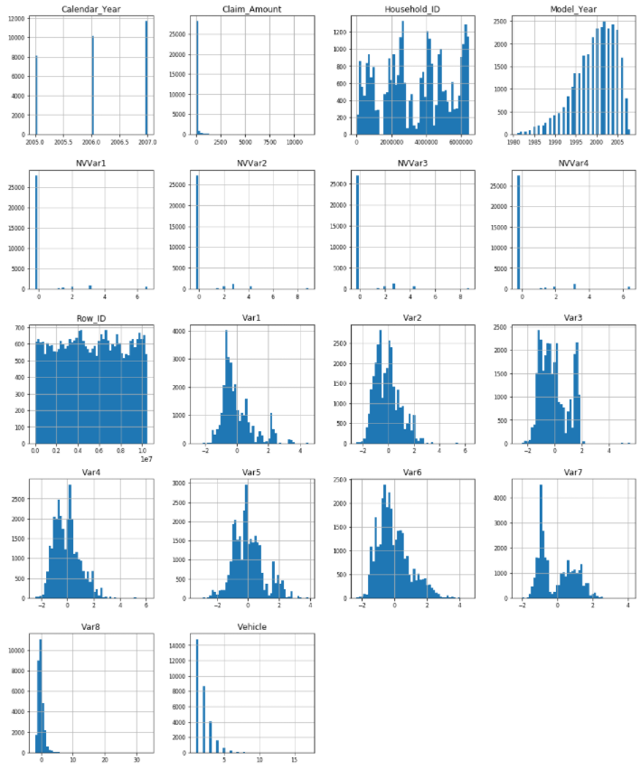

Visualising pairwise relationships in this dataset.

for i in range(0, len(df_num.columns), 5):
    sns.pairplot(data=df_num, x_vars=df_num.columns[i:i+5], y_vars=['Claim_Amount'])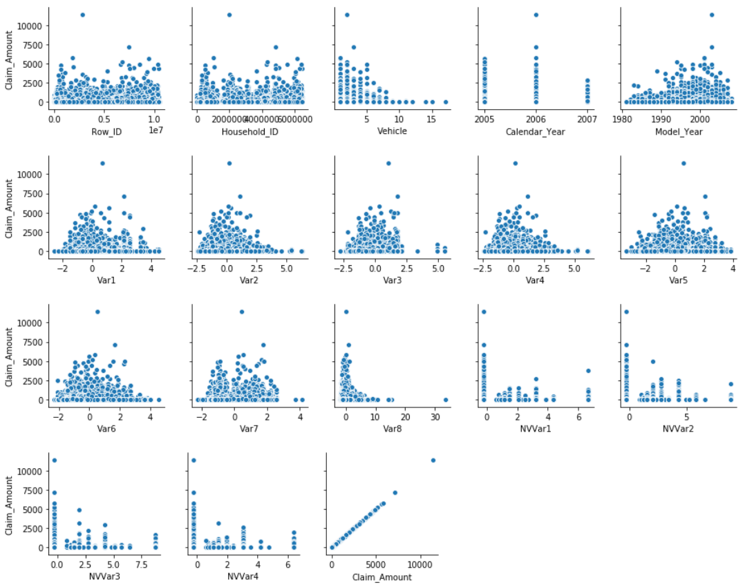

Review heatmaps among numerical types of data.

corr = df_num.drop('Claim_Amount', axis=1).corr()
plt.figure(figsize=(12, 10))
sns.heatmap(
    corr[(corr >= 0.5) | (corr <= -0.4)], 
    cmap='viridis', vmax=1.0, vmin=-1.0, linewidths=0.1,
    annot=True, annot_kws={"size": 8}, square=True);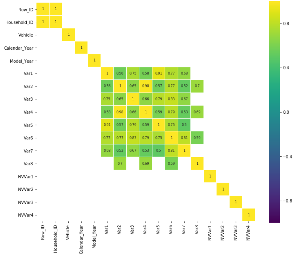

Categorical Types

While visualising categorical types of data, I saw there are some “?” in some features.

df_not_num = data.select_dtypes(include=['O'])
fig, axes = plt.subplots(round(len(df_not_num.columns) / 3), 3, figsize=(12, 20))
for i, ax in enumerate(fig.axes):
    if i < len(df_not_num.columns):
        ax.set_xticklabels(ax.xaxis.get_majorticklabels(), rotation=45)
        sns.countplot(x=df_not_num.columns[i], alpha=0.7, data=df_not_num, ax=ax)
fig.tight_layout()
plt.show()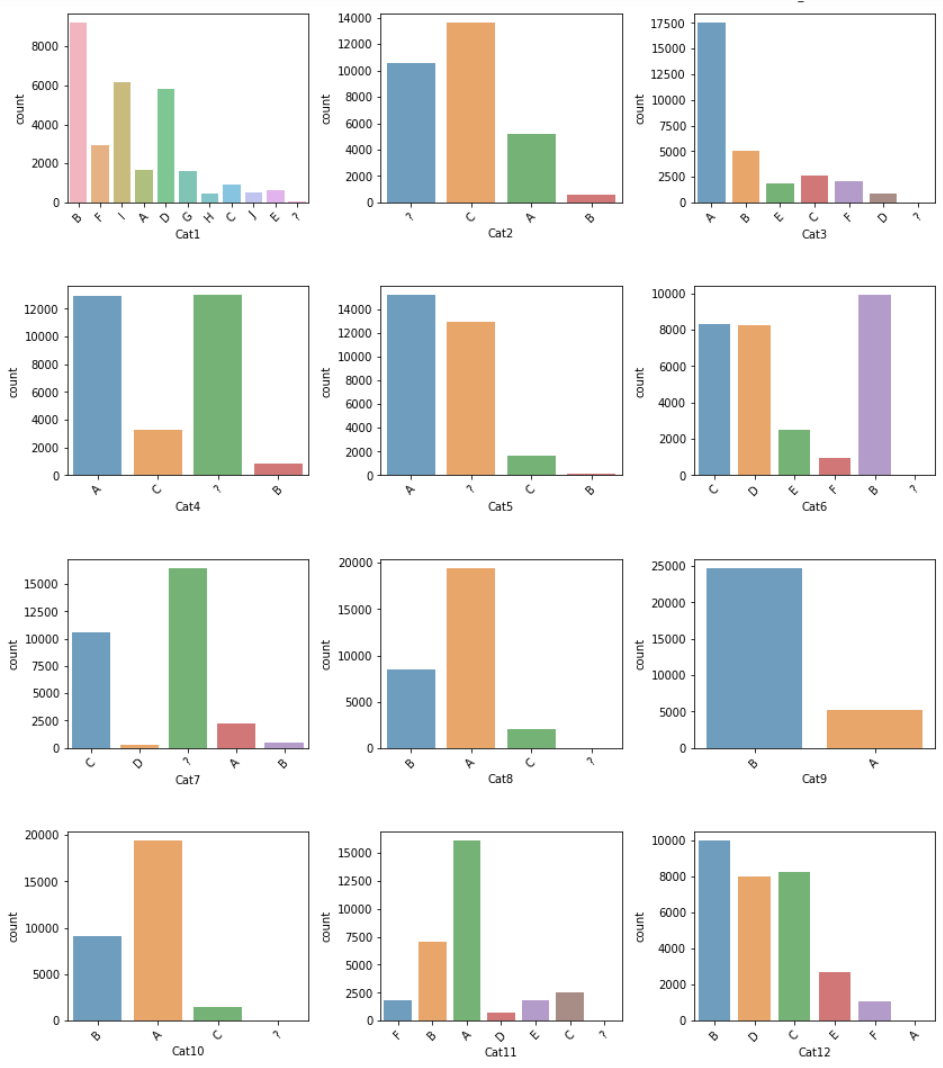

Feature Selection

Feature Selection is the process where you automatically or manually select those features which contribute most to your prediction variable or output in which you are interested in.

Feature \ Label	Continuous	Categorical
Continuous	Pearson’s Correlation	LDA
Categorical	ANOVA	Chi-Square

Featrue Selection using Chi-Square Test

The Chi-Square test of independence is a statistical test to determine if there is a significant relationship between 2 categorical variables. In simple words, the Chi-Square statistic will test whether there is a significant difference in the observed vs the expected frequencies of both variables.

import scipy.stats as stats
from scipy.stats import chi2_contingency

class ChiSquare:
    """"
    H0: No association between two variables.
    H1: There is evidence to suggest there is an association between two variables.
    """
    def __init__(self, data):
        self.data = data
        self.p_value = None
        self.chi2 = None
        self.dof = None
        self.data_observed = None
        self.data_expected = None
        self.important_features = []
        self.unimportant_features = []
        
    def print_result(self, col, alpha=0.05):
        if self.p_value < alpha:
            # Reject null hypothesis H0
            print(f"{col} is an IMPORTANT feature.")
        else:
            # Accept null hypothesis H0
            print(f"{col} is NOT an IMPORTANT feature.")
    
    def get_result(self, col, alpha=0.05):
        if self.p_value < alpha:
            # Reject null hypothesis H0
            self.important_features.append(col)
        else:
            # Accept null hypothesis H0
            self.unimportant_features.append(col)
    
    def get_important_features(self):
        return self.important_features
    
    def get_unimportant_features(self):
        return self.unimportant_features
        
    def test(self, col_features, col_y, alpha=0.05):
        for col_x in col_features:
            X = self.data[col_x].astype(str)
            y = self.data[col_y].apply(lambda label: 0 if label==0.0 else 1).astype(str)

            self.data_observed = pd.crosstab(y, X)
            chi2, p_value, dof, expected = chi2_contingency(self.data_observed.values)
            self.chi2 = chi2
            self.p_value = p_value
            self.dof = dof
            self.data_expected = pd.DataFrame(
                expected, 
                columns=self.data_observed.columns, 
                index=self.data_observed.index)
            self.get_result(col_x, alpha)
            self.print_result(col_x, alpha)

Chi-Square Test for Categorical Features.

chi_test = ChiSquare(data)
test_cols = df_not_num.columns.tolist()
chi_test.test(test_cols, "Claim_Amount")
important_cat_features = chi_test.get_important_features()
unimportant_cat_features = chi_test.get_unimportant_features()

---

Blind_Make is an IMPORTANT feature.
Blind_Model is an IMPORTANT feature.
Blind_Submodel is NOT an IMPORTANT feature.
Cat1 is an IMPORTANT feature.
Cat2 is an IMPORTANT feature.
Cat3 is an IMPORTANT feature.
Cat4 is an IMPORTANT feature.
Cat5 is an IMPORTANT feature.
Cat6 is an IMPORTANT feature.
Cat7 is an IMPORTANT feature.
Cat8 is NOT an IMPORTANT feature.
Cat9 is an IMPORTANT feature.
Cat10 is NOT an IMPORTANT feature.
Cat11 is NOT an IMPORTANT feature.
Cat12 is NOT an IMPORTANT feature.
OrdCat is an IMPORTANT feature.
NVCat is an IMPORTANT feature.

You can find out that ‘Blind_Make’, ‘Blind_Model’, ‘Cat1’, ‘Cat2’, ‘Cat3’, ‘Cat4’, ‘Cat5’, ‘Cat6’, ‘Cat7’, ‘Cat9’, ‘OrdCat’, ‘NVCat’ are important features, and ‘Blind_Submodel’, ‘Cat8’, ‘Cat10’, ‘Cat11’, ‘Cat12’ are unimportant features by Chi-Square Test.

Feature Selection using XGBoost

import xgboost as xgb
from xgboost import XGBClassifier
from xgboost import plot_importance
from sklearn.metrics import f1_score

def model(X_train, y_train, n_splits=3):
    scores=[]
    params = {
        'colsample_bytree': 0.8,                 
        'learning_rate': 0.08,
        'max_depth': 10,
        'subsample': 1,
        'objective': 'multi:softprob',
        'num_class': 2,
        'eval_metric': 'mlogloss',
        'min_child_weight': 3,
        'gamma': 0.25,
    }
    
    kf = StratifiedKFold(n_splits=n_splits, shuffle=True, random_state=42)
    for train_index, val_index in kf.split(X_train, y_train):
        train_X = X_train.iloc[train_index]
        val_X = X_train.iloc[val_index]
        train_y = y_train[train_index]
        val_y = y_train[val_index]
        xgb_train = xgb.DMatrix(train_X, train_y)
        xgb_eval = xgb.DMatrix(val_X, val_y)

        xgb_model = xgb.train(
            params,
            xgb_train,
            num_boost_round=1000,
            evals=[(xgb_train, 'train'), (xgb_eval, 'val')],
            verbose_eval=False,
            early_stopping_rounds=20
            )

        val_X = xgb.DMatrix(val_X)
        pred_val = [np.argmax(x) for x in xgb_model.predict(val_X)]
        score = f1_score(pred_val, val_y)
        scores.append(score)
        print('F1 score: ', score)

    return xgb_model

num_feature = [
        'Vehicle', 'Calendar_Year', 'Model_Year', 'Var1', 'Var2', 'Var3', 
        'Var4', 'Var5', 'Var6', 'Var7', 'Var8', 'NVVar1', 'NVVar2', 'NVVar3', 'NVVar4']
xgb_model = model(data[num_feature], (data.Claim_Amount!=0).astype(int), n_splits=5)

fig, ax = plt.subplots(figsize=(10, 10))
xgb.plot_importance(xgb_model, max_num_features=50, height=0.5, ax=ax, importance_type='gain',show_values=False)
plt.show()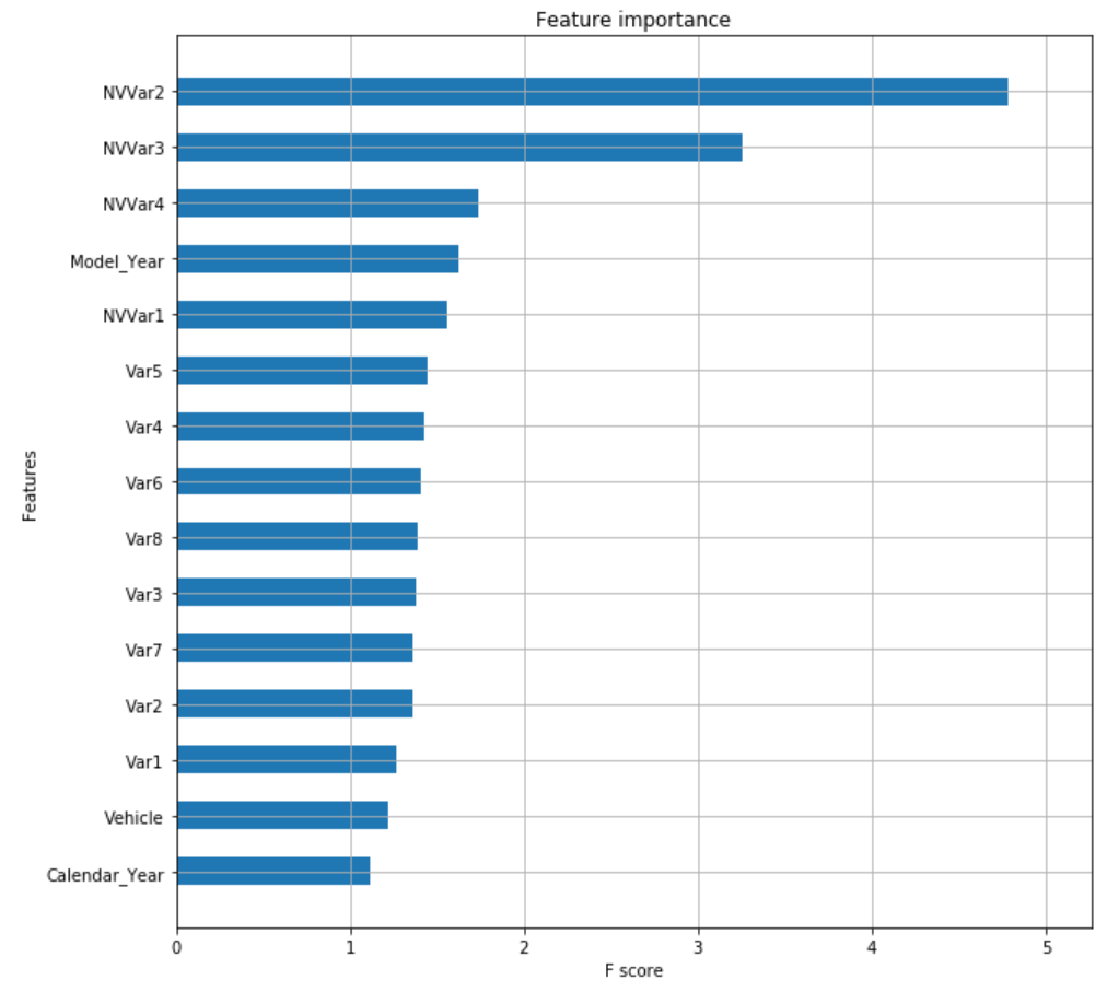

Missing Data

In this dataset, missing data is represented by a ‘?’ or a missing value. Therefore, it should start with tackling missing data. First, fill all None and missing data with np.nan. Second, replace ‘?’ by np.nan. Finally, plot a heatmap to get a view over the dataset.

def plot_missing_value_heatmap(data):
    plt.figure(figsize=(15, 10))
    sns.heatmap(data.isnull(), cbar=True, cmap=sns.color_palette("cubehelix"))
    plt.title("Missing Values Heatmap", fontdict={'family': 'serif', 'weight': 'normal', 'size': 16,})
    plt.show()

data_pre = data.copy()
data_pre.fillna(value=np.nan, inplace=True)
for col in object_features:
    data_pre.loc[:, col] = data_pre.loc[:, col].replace(to_replace='?',value=np.nan)
    data_pre.loc[:, col] = data_pre.loc[:, col].replace(to_replace='""',value=np.nan)
plot_missing_value_heatmap(data_pre)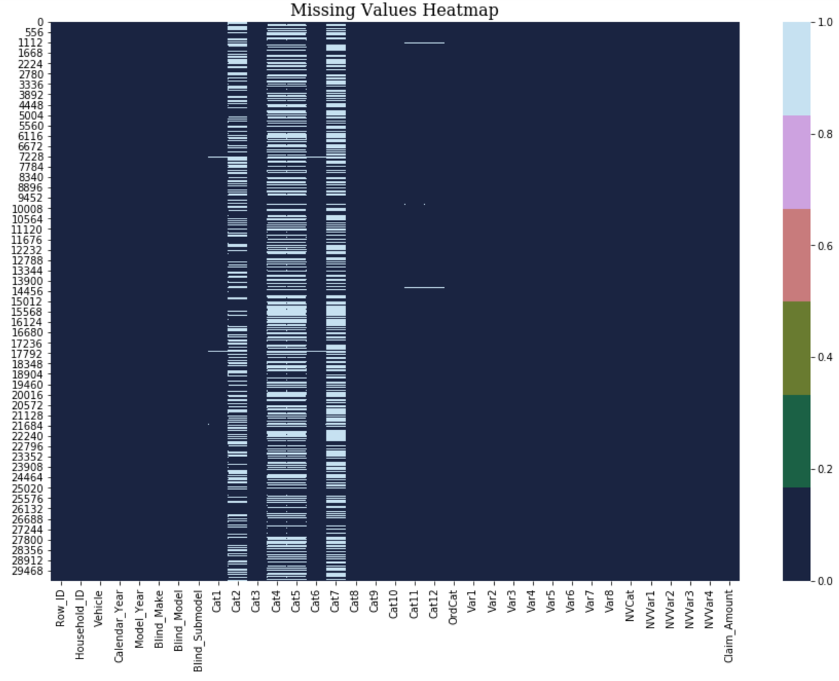

There are too many missing values in columns below:

• Cat2
• Cat4
• Cat5
• Cat7

So I just drop those columns.

# Split data into features and label
data_pre_feature1 = data_pre.drop('Claim_Amount', axis=1)
data_pre_label = data_pre['Claim_Amount']
# Convert int dtype into float dtype
for col in int_features:
    data_pre_feature1[col] = data_pre_feature1[col].astype('float64')
data_pre_feature1 = data_pre_feature1.drop(["Cat2", "Cat4", "Cat5", "Cat7"], axis=1)
plot_missing_value_heatmap(data_pre_feature1)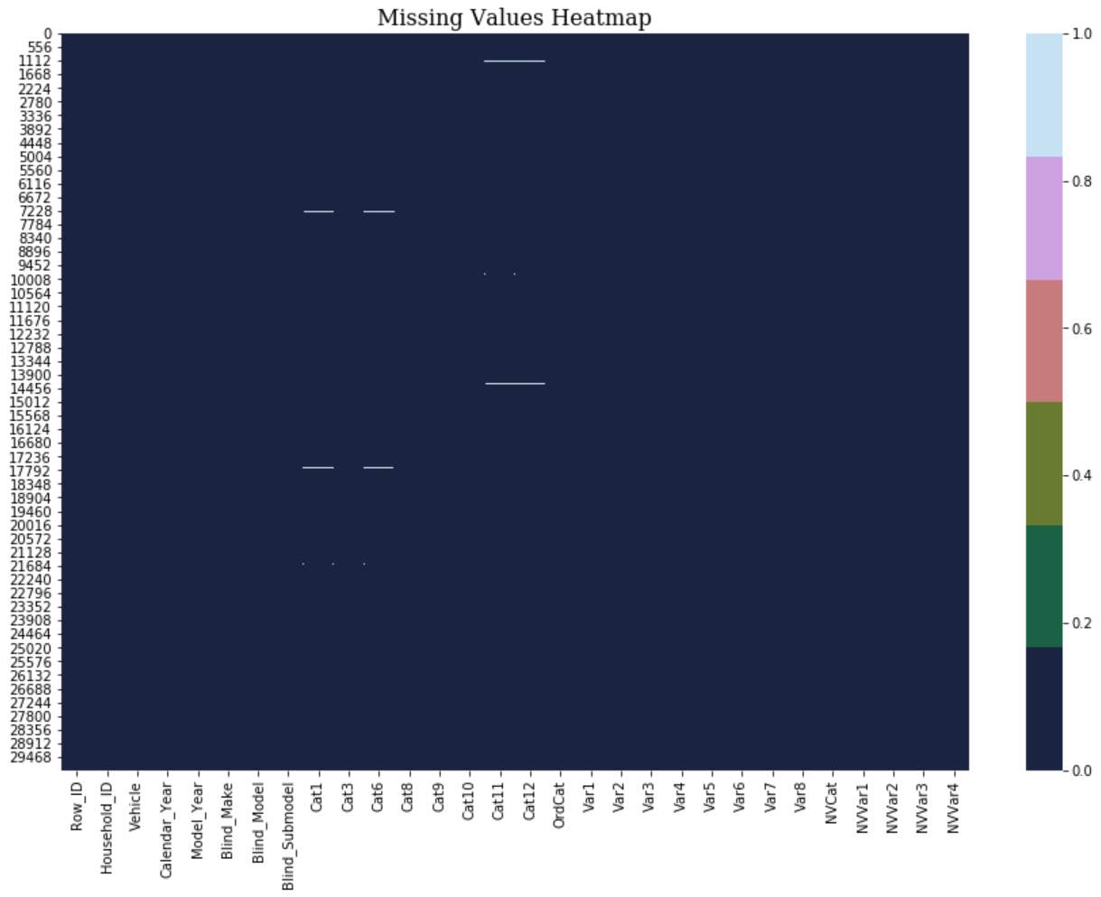

It’s quite good after removing these four columns! Therefore, for those features (“Cat2”, “Cat4”, “Cat5”, “Cat7”) which have more than 90% of missing value, I chose dropping them instead of filling . Rest of the featuers I chose using forward filling method from pandas library.

Features Transformation

I utilised different transformation methods for different data types.

1. ‘Blind_Make’, ‘Blind_Model’, ‘Blind_Submodel’: MeanEncoder() for high-cardinality categorical data.
2. ‘Row_ID’, ‘Household_ID’, ‘Vehicle’, ‘Calendar_Year’, ‘Model_Year’, ‘Var1’, ‘Var2’, ‘Var3’, ‘Var4’, ‘Var5’, ‘Var6’, ‘Var7’, ‘Var8’, ‘NVVar1’, ‘NVVar2’, ‘NVVar3’, ‘NVVar4’: MinMaxScaler() for numerical dat.
3. ‘Cat1’, ‘Cat3’, ‘Cat6’, ‘Cat8’, ‘Cat9’, ‘Cat10’, ‘Cat11’, ‘Cat12’, ‘OrdCat’, ‘NVCat’: OneHotEncoder() for categorical data (but in smaller dimension).

data_pre_feature2 = data_pre_feature1.fillna(method='ffill')
num_feature = [
    'Row_ID', 'Household_ID', 'Vehicle', 'Calendar_Year', 'Model_Year', 'Var1', 'Var2', 'Var3', 
    'Var4', 'Var5', 'Var6', 'Var7', 'Var8', 'NVVar1', 'NVVar2', 'NVVar3', 'NVVar4']
cat_feature = [
    'Cat1', 'Cat3', 'Cat6', 'Cat8', 'Cat9', 'Cat10', 'Cat11', 'Cat12', 'OrdCat', 'NVCat']
full_transform = ColumnTransformer([
    ("num", StandardScaler(), num_feature),
    ("cat", OneHotEncoder(), cat_feature)
])
data_pre_feature3 = full_transform.fit_transform(data_pre_feature2)

Mean Encoder

Mean Encoding is a simple preprocessing scheme for high-cardinality categorical data that allows this class of attributes to be used in predictive models such as neural networks, linear and logistic regression. The proposed method is based on a well-established statistical method (empirical Bayes) that is straightforward to implement as an in-database procedure. Furthermore, for categorical attributes with an inherent hierarchical structure, like ZIP codes, the preprocessing scheme can directly leverage the hierarchy by blending statistics at the various levels of aggregation.

I made this MeanEncoder() into sklearn-compatible class object.

class MeanEncoder(TransformerMixin, BaseEstimator):
    """
    http://helios.mm.di.uoa.gr/~rouvas/ssi/sigkdd/sigkdd.vol3.1/barreca.pdf
    """
    def __init__(self, cat_features, cv=10, target_type='classification', weight_func=None, k=2, f=1):
        self.cat_features = cat_features
        self.cv = cv
        self.k = k
        self.f = f
        self.learned_stats = {}
        if target_type == 'classification':
            self.target_type = target_type
            self.target_values = []
        elif target_type == 'regression':
            self.target_type = 'regression'
            self.target_values = None
        else:
            print("Label type could only be 'classification' or 'regression'.")
        # Calculate smoothing factor: 1 / (1 + np.exp(- (counts - min_samples_leaf) / smoothing_slope))
        if isinstance(weight_func, dict):
            self.weight_func = eval(
                'lambda x: 1 / (1 + np.exp(-(x-k)/f))', dict(weight_func, np=np, k=k, f=f))
        elif callable(weight_func):
            self.weight_func = weight_func
        else:
            self.weight_func = lambda x: 1 / (1 + np.exp(-(x-k)/f))

    # For training dataset
    def fit_transform(self, X, y):
        X_new = X.copy()
        if self.target_type == 'classification':
            skf = StratifiedKFold(self.cv)
        else:
            skf = KFold(self.cv)
        # Categorical label
        if self.target_type == 'classification':
            self.target_values = sorted(set(y))
            self.learned_stats = {'{}_pred_{}'.format(variable, target): [] for variable, target in
                                  product(self.cat_features, self.target_values)}
            for variable, target in product(self.cat_features, self.target_values):
                nf_name = '{}_pred_{}'.format(variable, target)
                X_new.loc[:, nf_name] = np.nan
                for large_ind, small_ind in skf.split(y, y):
                    nf_large, nf_small, prior, col_avg_y = MeanEncoder.mean_encode_blended(
                        X_new.iloc[large_ind], 
                        y.iloc[large_ind], 
                        X_new.iloc[small_ind], 
                        variable, 
                        target, 
                        self.weight_func)
                    X_new.iloc[small_ind, -1] = nf_small
                    self.learned_stats[nf_name].append((prior, col_avg_y))
        # Continuous label
        else:
            self.learned_stats = {'{}_pred'.format(variable): [] for variable in self.cat_features}
            for variable in self.cat_features:
                nf_name = '{}_pred'.format(variable)
                X_new.loc[:, nf_name] = np.nan
                for large_ind, small_ind in skf.split(y, y):
                    nf_large, nf_small, prior, col_avg_y = MeanEncoder.mean_encode_blended(
                        X_new.iloc[large_ind], 
                        y.iloc[large_ind], 
                        X_new.iloc[small_ind], 
                        variable, 
                        None, 
                        self.weight_func)
                    X_new.iloc[small_ind, -1] = nf_small
                    self.learned_stats[nf_name].append((prior, col_avg_y))
        X_new = X_new.drop(self.cat_features, axis=1)
        X_new.columns = self.cat_features
        return X_new

    # For testing dataset
    def transform(self, X):
        X_new = X.copy()
        # Categorical label
        if self.target_type == 'classification':
            for variable, target in product(self.cat_features, self.target_values):
                nf_name = '{}_pred_{}'.format(variable, target)
                X_new[nf_name] = 0
                for prior, col_avg_y in self.learned_stats[nf_name]:
                    X_new[nf_name] += X_new[[variable]].join(
                        col_avg_y, on=variable).fillna(prior, inplace=False)[
                        nf_name]
                X_new[nf_name] /= self.cv
        # Continuous label
        else:
            for variable in self.cat_features:
                nf_name = '{}_pred'.format(variable)
                X_new[nf_name] = 0
                for prior, col_avg_y in self.learned_stats[nf_name]:
                    X_new[nf_name] += X_new[[variable]].join(
                        col_avg_y, on=variable).fillna(prior, inplace=False)[
                        nf_name]
                X_new[nf_name] /= self.cv
        X_new = X_new.drop(self.cat_features, axis=1)
        X_new.columns = self.cat_features
        return X_new

    # Prior probability and posterior probability
    @staticmethod
    def mean_encode_blended(X_train, y_train, X_test, variable, target, weight_func):
        """
        S_i represents an estimate of the probability of Y=1 given X=X_i
        """
        X_train = X_train[[variable]].copy()
        X_test = X_test[[variable]].copy()

        if target is not None:
            nf_name = '{}_pred_{}'.format(variable, target)
            X_train['pred_temp'] = (y_train == target).astype(int)
        else:
            nf_name = '{}_pred'.format(variable)
            X_train['pred_temp'] = y_train
        # prior = n_Y / n_TR
        prior = X_train['pred_temp'].mean()
        # S_i['mean'] = n_iY/n_i and S_i['beta'] = lambda(n_i)
        S_i = X_train.groupby(by=variable, axis=0)['pred_temp'].agg(mean="mean", beta="size")
        S_i['beta'] = weight_func(S_i['beta'])
        # Empirical Bayes Estimation: S_i = lambda(n_i)*n_iY/n_i + (1-lambda(n_i))*n_Y/n_TR
        S_i[nf_name] = S_i['beta'] * S_i['mean'] + (1 - S_i['beta']) * prior
        S_i.drop(['beta', 'mean'], axis=1, inplace=True)
        nf_train = X_train.join(S_i, on=variable)[nf_name].values
        nf_test = X_test.join(S_i, on=variable).fillna(prior, inplace=False)[nf_name].values
        return nf_train, nf_test, prior, S_i

    def get_params(self, deep=True):
        return {
            "cat_features": self.cat_features, 
            "target_type": self.target_type, 
            "cv": self.cv, 
            "k": self.k, 
            "f": self.f}

    def set_params(self, **parameters):
        for parameter, value in parameters.items():
            setattr(self, parameter, value)
        return self

Perform MeanEncoder() on ‘Blind_Make’, ‘Blind_Model’, ‘Blind_Submodel’

# High-cardinality categorical data
mean_encoder_feature = ['Blind_Make', 'Blind_Model', 'Blind_Submodel']
me = MeanEncoder(cat_features=mean_encoder_feature, cv=10, target_type='regression')
data_pre_feature4 = me.fit_transform(data_pre[mean_encoder_feature], data_pre["Claim_Amount"])
data_pre_feature4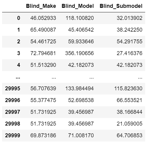

Imbalanced Data

The data is highly imbalanced: more records contain zero claims than not. When designing your predictive model, you need to account for this.

There are a couple of ways to deal with imbalanced data.

1. Resampling
2. Over-sampling: SMOTE
3. Under-sampling: Clustering, Tomek links

I built up-sampling and down-sampling functions to see whether they can improve the model.

from sklearn.utils import resample
from imblearn.pipeline import Pipeline
from imblearn.over_sampling import SMOTE
from imblearn.under_sampling import RandomUnderSampler

zero_label_num = len(data_pre_label[data_pre_label==0])
non_zero_label_num = len(data_pre_label[data_pre_label>0])

def upsampling(features, labels):
    df = pd.concat([features, labels], axis=1)
    # Separate majority and minority classes
    df_majority = df[df.Claim_Amount==0]
    df_minority = df[df.Claim_Amount!=0]
    # Upsample minority class
    df_minority_upsampled = resample(df_minority, replace=True, n_samples=df_majority.shape[0], random_state=914)
    # Combine majority class with upsampled minority class
    df_upsampled = pd.concat([df_majority, df_minority_upsampled])
    # Display new class counts
    print(
        f"Non zero: {len(df_upsampled[df_upsampled.Claim_Amount>0])} \
        Zero: {len(df_upsampled[df_upsampled.Claim_Amount==0])}")
    return df_upsampled.drop('Claim_Amount', axis=1), df_upsampled.Claim_Amount

def downsampling(features, labels):
    df = pd.concat([features, labels], axis=1)
    # Separate majority and minority classes
    df_majority = df[df.Claim_Amount==0]
    df_minority = df[df.Claim_Amount!=0]
    # Downsample majority class
    df_majority_downsampled = resample(df_majority, replace=False, n_samples=df_minority.shape[0], random_state=411)
    # Combine minority class with downsampled majority class
    df_downsampled = pd.concat([df_majority_downsampled, df_minority])
    # Display new class counts
    print(
        f"Non zero: {len(df_downsampled[df_downsampled.Claim_Amount>0])} \
        Zero: {len(df_downsampled[df_downsampled.Claim_Amount==0])}")
    return df_downsampled.drop('Claim_Amount', axis=1), df_downsampled.Claim_Amount

def smote_sampling(X, y):
    smote = SMOTE(sampling_strategy="minority")
    X, y = smote.fit_resample(X, y)
    return X, y

Put it all together!

def preprocessing_baseline(dataframe, use_upsampling=None, use_downsampling=None):
    # Split into training and validation
    data = dataframe.copy()
    X_train, X_valid, y_train, y_valid = train_test_split(
        data.drop("Claim_Amount", axis=1), 
        data.Claim_Amount, 
        test_size=0.15, 
        random_state=42, 
        stratify=(data.Claim_Amount!=0).astype(int))
    if use_upsampling == True: X_train, y_train = upsampling(X_train, y_train)
    if use_downsampling == True: X_train, y_train = downsampling(X_train, y_train)
    # Define different datatype
    int_features, float_features, object_features = type_of_col(data, label_col='Claim_Amount', show=False)
    # ========================================
    #               Training
    # ========================================
    X_train.fillna(value=np.nan, inplace=True)
    # Replace ? with np.nan
    for col in object_features:
        X_train.loc[:, col] = X_train.loc[:, col].replace(to_replace='?',value=np.nan)
        X_train.loc[:, col] = X_train.loc[:, col].replace(to_replace='""',value=np.nan)
    # Convert int to float
    for col in int_features:
        X_train[col] = X_train[col].astype('float64')
    X_train = X_train.fillna(method='ffill')
    full_transform = ColumnTransformer([
        ("num", StandardScaler(), int_features+float_features),
        ("cat", OneHotEncoder(), object_features)
    ])
    X_train = full_transform.fit_transform(X_train)
    # ========================================
    #               Validation
    # ========================================
    X_valid.fillna(value=np.nan, inplace=True)
    # Replace ? with np.nan
    for col in object_features:
        X_valid.loc[:, col] = X_valid.loc[:, col].replace(to_replace='?',value=np.nan)
    # Convert int to float
    for col in int_features:
        X_valid[col] = X_valid[col].astype('float64')
    X_valid = X_valid.fillna(method='ffill')
    X_valid = full_transform.transform(X_valid)
    print(f"Size of training feature: {X_train.shape}\nSize of validation feature: {X_valid.shape}")
    print(f"Size of training label: {y_train.shape}\nSize of validation label: {y_valid.shape}")
    return X_train, X_valid, y_train, y_valid, full_transform
    
def preprocessing_v2(dataframe, use_upsampling=None, use_downsampling=None, use_blended=None):
    # Split into training and validation
    data = dataframe.copy()
    X_train, X_valid, y_train, y_valid = train_test_split(
        data.drop("Claim_Amount", axis=1), 
        data.Claim_Amount, 
        test_size=0.15, 
        random_state=42, 
        stratify=(data.Claim_Amount!=0).astype(int))
    if use_upsampling == True: X_train, y_train = upsampling(X_train, y_train)
    if use_downsampling == True: X_train, y_train = downsampling(X_train, y_train)
    # Define different datatype
    mean_encoder_feature = [
        'Blind_Make', 'Blind_Model', 'Blind_Submodel']
    num_feature = [
        'Vehicle', 'Calendar_Year', 'Model_Year', 'Var1', 'Var2', 'Var3', 
        'Var4', 'Var5', 'Var6', 'Var7', 'Var8', 'NVVar1', 'NVVar2', 'NVVar3', 'NVVar4']
    onehot_feature = [
        'Cat1', 'Cat3', 'Cat6', 'Cat8', 'Cat9', 'Cat10', 'Cat11', 'Cat12', 'OrdCat', 'NVCat']
    # ========================================
    #               Training
    # ========================================
    X_train = X_train.drop(['Row_ID', 'Household_ID', "Cat2", "Cat4", "Cat5", "Cat7"], axis=1)
    X_train.fillna(value=np.nan, inplace=True)
    # Replace ? and "" with np.nan
    for col in onehot_feature:
        X_train.loc[:, col] = X_train.loc[:, col].replace(to_replace='?',value=np.nan)
        X_train.loc[:, col] = X_train.loc[:, col].replace(to_replace='""',value=np.nan)
    # Convert int to float
    for col in num_feature:
        X_train[col] = X_train[col].astype('float64')
    X_train = X_train.fillna(method='ffill')
    full_transform = ColumnTransformer([
        ("num", MinMaxScaler(), num_feature),
        ("cat", OneHotEncoder(), onehot_feature), 
        ("mean", MeanEncoder(cat_features=mean_encoder_feature, target_type="regression"), mean_encoder_feature)
    ])
    X_train_final = full_transform.fit_transform(X_train, y_train)
    # ========================================
    #               Validation
    # ========================================
    X_valid = X_valid.drop(['Row_ID', 'Household_ID', "Cat2", "Cat4", "Cat5", "Cat7"], axis=1)
    X_valid.fillna(value=np.nan, inplace=True)
    # Replace ? and "" with np.nan
    for col in onehot_feature:
        X_valid.loc[:, col] = X_valid.loc[:, col].replace(to_replace='?',value=np.nan)
        X_valid.loc[:, col] = X_valid.loc[:, col].replace(to_replace='""',value=np.nan)
    # Convert int to float
    for col in num_feature:
        X_valid[col] = X_valid[col].astype('float64')
    X_valid = X_valid.fillna(method='ffill')
    X_valid_final = full_transform.transform(X_valid)
    print(f"Size of training data: {X_train_final.shape}\nSize of validation data: {X_valid_final.shape}")
    print(f"Size of training label: {y_train.shape}\nSize of validation label: {y_valid.shape}")
    return X_train_final, X_valid_final, y_train, y_valid, full_transform

def preprocessing_v3(dataframe, use_upsampling=None, use_downsampling=None, use_blended=None):
    # Define different datatype
    label = ["Claim_Amount"]
    mean_encoder_feature = ['Blind_Make', 'Blind_Model']
    num_feature = ['Var1', 'Var6', 'NVVar1', 'NVVar2', 'NVVar3', 'NVVar4']
    onehot_feature = ['Cat1', 'Cat3', 'Cat6', 'Cat9', 'OrdCat', 'NVCat']
    # Split into training and validation
    data = dataframe.copy()
    data = data[mean_encoder_feature+num_feature+onehot_feature+label]
    X_train, X_valid, y_train, y_valid = train_test_split(
        data.drop("Claim_Amount", axis=1), 
        data.Claim_Amount, 
        test_size=0.15, 
        random_state=42, 
        stratify=(data.Claim_Amount!=0).astype(int))
    if use_upsampling == True: X_train, y_train = upsampling(X_train, y_train)
    if use_downsampling == True: X_train, y_train = downsampling(X_train, y_train)
    # ========================================
    #               Training
    # ========================================
    X_train.fillna(value=np.nan, inplace=True)
    # Replace ? and "" with np.nan
    for col in onehot_feature:
        X_train.loc[:, col] = X_train.loc[:, col].replace(to_replace='?',value=np.nan)
        X_train.loc[:, col] = X_train.loc[:, col].replace(to_replace='""',value=np.nan)
    # Convert int to float
    for col in num_feature:
        X_train[col] = X_train[col].astype('float64')
    X_train = X_train.fillna(method='ffill')
    full_transform = ColumnTransformer([
        ("num", MinMaxScaler(), num_feature),
        ("cat", OneHotEncoder(), onehot_feature), 
        ("mean", MeanEncoder(cat_features=mean_encoder_feature, target_type="regression"), mean_encoder_feature)
    ])
    X_train_final = full_transform.fit_transform(X_train, y_train)
    # ========================================
    #               Validation
    # ========================================
    X_valid.fillna(value=np.nan, inplace=True)
    # Replace ? and "" with np.nan
    for col in onehot_feature:
        X_valid.loc[:, col] = X_valid.loc[:, col].replace(to_replace='?',value=np.nan)
        X_valid.loc[:, col] = X_valid.loc[:, col].replace(to_replace='""',value=np.nan)
    # Convert int to float
    for col in num_feature:
        X_valid[col] = X_valid[col].astype('float64')
    X_valid = X_valid.fillna(method='ffill')
    X_valid_final = full_transform.transform(X_valid)
    print(f"Size of training data: {X_train_final.shape}\nSize of validation data: {X_valid_final.shape}")
    print(f"Size of training label: {y_train.shape}\nSize of validation label: {y_valid.shape}")
    return X_train_final, X_valid_final, y_train, y_valid, full_transform

Modelling

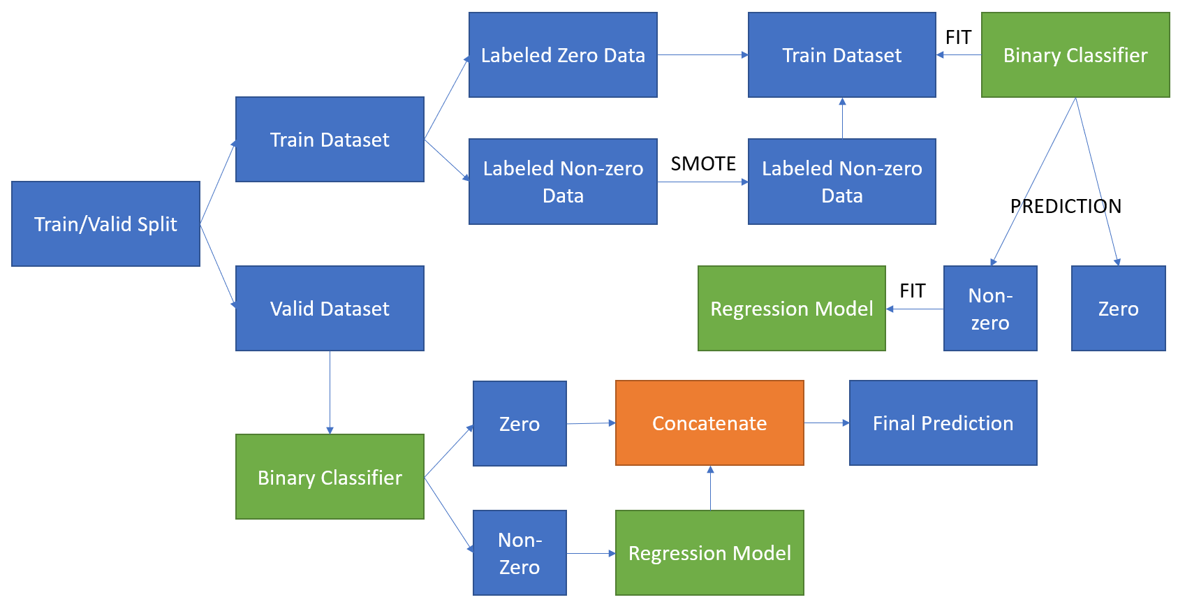
Tandem Model

Tandem is a two-stage regression method that can be used when various input data types are correlated, for example gene expression and methylation in drug response prediction. In the first stage it uses the upstream features (such as methylation) to predict the response variable (such as drug response), and in the second stage it uses the downstream features (such as gene expression) to predict the residuals of the first stage.

Pipeline

Performance using Single Model

You can see the problem as a regression problem where the variable to predict is continuous (the claimed amount in USD). The performance of the regression model will depend on the quality of the training data. I’ll compare the performance of the following models:

1. Linear regression
2. Ridge regression
3. Random forests for regression
4. Gradient tree boosting for regression

For each model, I’ll use grid search with at least three options for each parameter and report the performance measure over a validation set.

from sklearn.metrics import mean_squared_error
from sklearn.decomposition import TruncatedSVD
from sklearn.linear_model import LinearRegression
from sklearn.linear_model import Ridge
from sklearn.ensemble import RandomForestRegressor
from sklearn.ensemble import GradientBoostingRegressor
from sklearn.model_selection import train_test_split
from sklearn.model_selection import GridSearchCV
from sklearn.model_selection import learning_curve

Let’s split our data into training and validation dataset using preprocessing_v2() we built above.

X_train, X_valid, y_train, y_valid, _ = preprocessing_v2(data)

Main Code

Linear Regression

RMSE: 274.5014

"""
Best params: 
Origin: {'copy_X': True, 'fit_intercept': False, 'normalize': True}
Upsampling: {'copy_X': True, 'fit_intercept': True, 'normalize': False}
Downsampling: {'copy_X': True, 'fit_intercept': False, 'normalize': True}
"""
USE_GRID = False

if USE_GRID:
    param_grid = {
        'normalize': [True, False], 
        'fit_intercept': [True, False], 
        'copy_X': [True, False]
    }
    grid = GridSearchCV(LinearRegression(), cv=3, param_grid=param_grid, n_jobs=8)
    grid.fit(X_train, y_train)
    lr = grid.best_estimator_
    print(f"Best params: {grid.best_params_}")
    y_pred = lr.predict(X_valid)
    rmse = np.sqrt(mean_squared_error(y_valid, y_pred))
    print(f"RMSE: {round(rmse, 4)}")
else: 
    best_params = {
        'copy_X': True, 'fit_intercept': False, 'normalize': True
    }
    lr = LinearRegression(**best_params)
    lr.fit(X_train, y_train)
    y_pred = lr.predict(X_valid)
    rmse = np.sqrt(mean_squared_error(y_valid, y_pred))
    print(f"RMSE: {round(rmse, 4)}")

Ridge Regression

RMSE: 274.3249

"""
Best params: 
Origin: {'alpha': 1.0, 'fit_intercept': True, 'normalize': True}
Upsampling: {'alpha': 1.0, 'fit_intercept': True, 'normalize': False}
Downsampling: {'alpha': 1.0, 'fit_intercept': True, 'normalize': False}
"""
USE_GRID = False

if USE_GRID:
    param_grid = {
        'alpha': [float(x) for x in np.linspace(0.1, 1.0, 10)], 
        'fit_intercept': [True, False], 
        'normalize':[True, False]
    }
    grid = GridSearchCV(Ridge(), cv=3, param_grid=param_grid, n_jobs=8)
    grid.fit(X_train, y_train)
    rr = grid.best_estimator_
    print(f"Best params: {grid.best_params_}")
    y_pred = rr.predict(X_valid)
    rmse = np.sqrt(mean_squared_error(y_valid, y_pred))
    print(f"RMSE: {round(rmse, 4)}")
else: 
    best_params = {
        'alpha': 1.0, 'fit_intercept': True, 'normalize': True
    }
    rr = Ridge(**best_params)
    rr.fit(X_train, y_train)
    y_pred = rr.predict(X_valid)
    rmse = np.sqrt(mean_squared_error(y_valid, y_pred))
    print(f"RMSE: {round(rmse, 4)}")

---

def pretty_print_coefficients(coefficients, names=None, sort=False):
    if names == None:
        names = ["X{}".format(x) for x in range(len(coefficients))]
    lst = zip(coefficients, names)
    if sort:
        lst = sorted(lst, key=lambda x: -np.abs(x[0]))
    return " + ".join("%s * %s" % (round(coef, 3), name) for coef, name in lst)

pretty_print_coefficients(rr.coef_, names=None, sort=False)

---

'14.713 * X0 + -7.194 * X1 + 0.668 * X2 + 6.268 * X3 + 3.181 * X4 + 0.285 * X5 + 6.009 * X6 + 4.608 * X7 + -3.255 * X8 + 1.433 * X9 + -18.1 * X10 + -5.12 * X11 + 5.512 * X12 + -3.907 * X13 + -2.035 * X14 + -1.468 * X15 + 1.483 * X16 + -5.298 * X17 + 0.849 * X18 + -6.152 * X19 + -0.607 * X20 + 1.392 * X21 + 13.419 * X22 + -1.513 * X23 + -3.255 * X24 + 4.119 * X25 + -2.235 * X26 + -6.145 * X27 + -2.228 * X28 + -0.052 * X29 + -2.067 * X30 + -0.584 * X31 + 1.877 * X32 + 0.801 * X33 + -5.243 * X34 + -0.085 * X35 + 1.982 * X36 + -0.864 * X37 + -4.318 * X38 + -0.041 * X39 + 0.041 * X40 + 0.981 * X41 + -0.338 * X42 + -3.315 * X43 + 0.591 * X44 + 0.117 * X45 + 0.963 * X46 + 0.254 * X47 + -3.111 * X48 + -1.329 * X49 + 42.711 * X50 + -0.511 * X51 + 1.54 * X52 + 0.599 * X53 + -3.295 * X54 + -1.784 * X55 + 58.729 * X56 + -0.35 * X57 + -7.959 * X58 + 0.052 * X59 + 0.335 * X60 + -1.077 * X61 + -21.379 * X62 + 6.138 * X63 + -0.224 * X64 + 11.816 * X65 + -1.387 * X66 + 3.474 * X67 + -3.939 * X68 + -10.15 * X69 + -7.045 * X70 + -15.198 * X71 + -1.191 * X72 + -0.275 * X73 + -2.104 * X74 + 0.844 * X75 + 1.142 * X76 + -0.481 * X77 + 0.041 * X78 + -0.005 * X79 + -0.005 * X80'

Random Forest

RMSE: 274.4148

"""
Best params: 
Origin: {'max_depth': 3, 'min_samples_split': 10, 'n_estimators': 100}
Upsampling: {'max_depth': 5, 'min_samples_split': 5, 'n_estimators': 100}
Downsampling: {'max_depth': 5, 'min_samples_split': 5, 'n_estimators': 200}
"""
USE_GRID = False

if USE_GRID:
    param_grid = {
        'n_estimators': [int(x) for x in np.linspace(100, 300, 3)], 
        'max_depth': [int(x) for x in range(3, 6)], 
        'min_samples_split': [2, 5, 10], 
#     'min_samples_leaf': [1, 2, 4], 
#     'bootstrap': [True, False]
    }
    grid = GridSearchCV(RandomForestRegressor(), cv=3, param_grid=param_grid, n_jobs=8)
    grid.fit(X_train, y_train)
    rfr = grid.best_estimator_
    print(f"Best params: {grid.best_params_}")
    y_pred = rfr.predict(X_valid)
    rmse = np.sqrt(mean_squared_error(y_valid, y_pred))
    print(f"RMSE: {round(rmse, 4)}")
else: 
    best_params = {
        'max_depth': 3, 'min_samples_split': 10, 'n_estimators': 100
    }
    rfr = RandomForestRegressor(**best_params)
    rfr.fit(X_train, y_train)
    y_pred = rfr.predict(X_valid)
    rmse = np.sqrt(mean_squared_error(y_valid, y_pred))
    print(f"RMSE: {round(rmse, 4)}")

Gradient Tree Boosting

RMSE: 274.5765

"""
Best params: 
Origin: {'max_depth': 3, 'min_samples_split': 0.5, 'n_estimators': 200}
Upsampling: {'max_depth': 5, 'min_samples_split': 0.1, 'n_estimators': 500}
Downsampling: {'max_depth': 3, 'min_samples_split': 0.5, 'n_estimators': 200}
"""
USE_GRID = False

if USE_GRID:
    param_grid = {
        'n_estimators': [int(x) for x in np.linspace(200, 400, 3)], 
        'max_depth': [int(x) for x in range(3, 6)], 
        "min_samples_split": np.linspace(0.1, 0.5, 12), 
#     'learning_rate': [0.1, 0.01, 0.001], 
#     'min_samples_leaf': np.linspace(0.1, 0.5, 12), 
#     "subsample": [0.5, 0.618, 0.8, 0.85, 0.9, 0.95, 1.0], 
#     'max_features': ["log2","sqrt"]
    }
    grid = GridSearchCV(GradientBoostingRegressor(), cv=3, param_grid=param_grid, n_jobs=8)
    grid.fit(X_train, y_train)
    gbr = grid.best_estimator_
    print(f"Best params: {grid.best_params_}")
    y_pred = gbr.predict(X_valid)
    rmse = np.sqrt(mean_squared_error(y_valid, y_pred))
    print(f"RMSE: {round(rmse, 4)}")
else: 
    best_params = {
        'max_depth': 3, 'min_samples_split': 0.5, 'n_estimators': 200
    }
    gbr = GradientBoostingRegressor(**best_params)
    gbr.fit(X_train, y_train)
    y_pred = gbr.predict(X_valid)
    rmse = np.sqrt(mean_squared_error(y_valid, y_pred))
    print(f"RMSE: {round(rmse, 4)}")

Performance

from IPython.display import HTML, display

report = [
    ["", "RMSE (original)", "RMSE (up-sampling)", "RMSE (down-sampling)"],
    ["Linear Regression", 204.9581, 214.4630, 214.3920],
    ["Ridge Regression", 204.6595, 214.4686, 214.3732], 
    ["Random Forest", 204.6774, 221.9525, 233.0449], 
    ["Gradient Tree Boosting", 205.4188, 230.6640, 219.3338]
    ]
display(HTML(
   '<table><tr>{}</tr></table>'.format(
       '</tr><tr>'.join(
           '<td>{}</td>'.format('</td><td>'.join(str(_) for _ in row)) for row in report))))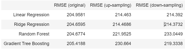

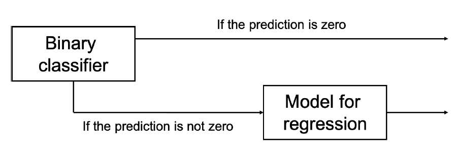
Performance using a combination of two models

In this section, I will build a prediction model based on two separate models in tandem (one after the other). The first model will be a binary classifier that will tell whether the claim was zero or different from zero. I will compare the following classifiers: random forests for classification and gradient boosting for classification.

As usual, load in required libraries.

from sklearn.ensemble import RandomForestClassifier
from sklearn.ensemble import GradientBoostingClassifier
from sklearn.metrics import confusion_matrix
from sklearn.metrics import classification_report

And split it into training and validation dataset using preprocessing_v2().

X_train, X_valid, y_train, y_valid, full_transform = preprocessing_v2(data)
y_train_binary = (y_train != 0.0).astype(int)
y_valid_binary = (y_valid != 0.0).astype(int)

Second Model

Random Forest

"""
Best params: 
Origin: {'max_depth': 3, 'min_samples_split': 2, 'n_estimators': 100}
Upsampling: {'max_depth': 9, 'min_samples_split': 7, 'n_estimators': 300}
Downsampling: {'max_depth': 9, 'min_samples_split': 7, 'n_estimators': 300}
"""
USE_GRID = False

if USE_GRID:
    param_grid = {
        'n_estimators': [int(x) for x in np.linspace(300, 500, 3)], 
        'max_depth': [int(x) for x in range(5, 10)], 
        'min_samples_split': [7, 9, 10]
    }
    grid = GridSearchCV(RandomForestClassifier(), cv=3, param_grid=param_grid, n_jobs=8, scoring="f1")
    grid.fit(X_train, y_train_binary)
    rfc = grid.best_estimator_
    print(f"Best params: {grid.best_params_}")
    y_pred = rfc.predict(X_valid)
else: 
    best_params = {
        'max_depth': 3, 'min_samples_split': 2, 'n_estimators': 100
    }
    rfc = RandomForestClassifier(**best_params)
    rfc.fit(X_train, y_train_binary)
    y_pred = rfc.predict(X_valid)
    
print(classification_report(y_valid_binary, y_pred))
print(confusion_matrix(y_valid_binary, y_pred))

Gradient Boosting

"""
Best params: 
Origin: {'max_depth': 3, 'min_samples_split': 0.30000000000000004, 'n_estimators': 300}
Upsampling: {'max_depth': 5, 'min_samples_split': 0.1, 'n_estimators': 400}
Downsampling: {'max_depth': 5, 'min_samples_split': 0.1, 'n_estimators': 300}
"""
USE_GRID = False

if USE_GRID:
    param_grid = {
        'n_estimators': [int(x) for x in np.linspace(200, 400, 3)], 
        'max_depth': [int(x) for x in range(3, 6)], 
        "min_samples_split": np.linspace(0.1, 0.5, 3), 
#     'learning_rate': [0.1, 0.01, 0.001], 
#     'min_samples_leaf': np.linspace(0.1, 0.5, 12), 
#     "subsample": [0.5, 0.618, 0.8, 0.85, 0.9, 0.95, 1.0], 
#     'max_features': ["log2","sqrt"]
    }
    grid = GridSearchCV(GradientBoostingClassifier(), cv=3, param_grid=param_grid, n_jobs=8, scoring="f1")
    grid.fit(X_train, y_train_binary)
    gbc = grid.best_estimator_
    print(f"Best params: {grid.best_params_}")
    y_pred = gbc.predict(X_valid)
else: 
    best_params = {
        'max_depth': 3, 'min_samples_split': 0.30000000000000004, 'n_estimators': 300
    }
    gbc = GradientBoostingClassifier(**best_params)
    gbc.fit(X_train, y_train_binary)
    y_pred = gbc.predict(X_valid)
    
print(classification_report(y_valid_binary, y_pred))
print(confusion_matrix(y_valid_binary, y_pred))

Put these two models as second model, and combine with primary model. For the second model, if the claim was different from zero, train a regression model to predict the actual value of the claim.

This time, I’ll put all code together inside a code block.

"""
Best params: 
Origin: {'copy_X': True, 'fit_intercept': False, 'normalize': True}
Upsampling: {'copy_X': True, 'fit_intercept': True, 'normalize': False}
Downsampling: {'copy_X': True, 'fit_intercept': True, 'normalize': True}
"""
USE_GRID = False

if USE_GRID:
    param_grid = {
        'normalize': [True, False], 
        'fit_intercept': [True, False], 
        'copy_X': [True, False]
    }
    grid = GridSearchCV(LinearRegression(), cv=3, param_grid=param_grid, n_jobs=8)
    grid.fit(X_train[np.where(y_train != 0)], y_train[y_train != 0])
    lr_2 = grid.best_estimator_
    print(f"Best params: {grid.best_params_}")
    y_pred = lr_2.predict(X_valid[np.where(y_valid != 0)])
    rmse = np.sqrt(mean_squared_error(y_valid[y_valid != 0], y_pred))
    print(f"RMSE: {round(rmse, 4)}")
else: 
    best_params = {
        'copy_X': True, 'fit_intercept': True, 'normalize': True
    }
    lr_2 = LinearRegression(**best_params)
    lr_2.fit(X_train[np.where(y_train != 0)], y_train[y_train != 0])
    y_pred = lr_2.predict(X_valid[np.where(y_valid != 0)])
    rmse = np.sqrt(mean_squared_error(y_valid[y_valid != 0], y_pred))
    print(f"RMSE: {round(rmse, 4)}")

"""
Best params: 
Origin: {'alpha': 1.0, 'fit_intercept': True, 'normalize': True}
Upsampling: {'alpha': 0.1, 'fit_intercept': True, 'normalize': True}
Downsampling: {'alpha': 1.0, 'fit_intercept': True, 'normalize': True}
"""
USE_GRID = False

if USE_GRID:
    param_grid = {
        'alpha': [float(x) for x in np.linspace(0.1, 1.0, 10)], 
        'fit_intercept': [True, False], 
        'normalize':[True, False]
    }
    grid = GridSearchCV(Ridge(), cv=3, param_grid=param_grid, n_jobs=8)
    grid.fit(X_train[np.where(y_train != 0)], y_train[y_train != 0])
    rr_2 = grid.best_estimator_
    print(f"Best params: {grid.best_params_}")
    y_pred = rr_2.predict(X_valid[np.where(y_valid != 0)])
    rmse = np.sqrt(mean_squared_error(y_valid[y_valid != 0], y_pred))
    print(f"RMSE: {round(rmse, 4)}")
else: 
    best_params = {
        'alpha': 1.0, 'fit_intercept': True, 'normalize': True
    }
    rr_2 = Ridge(**best_params)
    rr_2.fit(X_train[np.where(y_train != 0)], y_train[y_train != 0])
    y_pred = rr_2.predict(X_valid[np.where(y_valid != 0)])
    rmse = np.sqrt(mean_squared_error(y_valid[y_valid != 0], y_pred))
    print(f"RMSE: {round(rmse, 4)}")

"""
Best params: 
Origin: {'max_depth': 3, 'min_samples_split': 2, 'n_estimators': 100}
Upsampling: {'max_depth': 5, 'min_samples_split': 2, 'n_estimators': 300}
Downsampling: {'max_depth': 3, 'min_samples_split': 2, 'n_estimators': 300}
"""
USE_GRID = False

if USE_GRID:
    param_grid = {
        'n_estimators': [int(x) for x in np.linspace(100, 300, 3)], 
        'max_depth': [int(x) for x in range(3, 6)], 
        'min_samples_split': [2, 5, 10], 
#     'min_samples_leaf': [1, 2, 4], 
#     'bootstrap': [True, False]
    }
    grid = GridSearchCV(RandomForestRegressor(), cv=3, param_grid=param_grid, n_jobs=8)
    grid.fit(X_train[np.where(y_train != 0)], y_train[y_train != 0])
    rfr_2 = grid.best_estimator_
    print(f"Best params: {grid.best_params_}")
    y_pred = rfr_2.predict(X_valid[np.where(y_valid != 0)])
    rmse = np.sqrt(mean_squared_error(y_valid[y_valid != 0], y_pred))
    print(f"RMSE: {round(rmse, 4)}")
else: 
    best_params = {
        'max_depth': 3, 'min_samples_split': 2, 'n_estimators': 100
    }
    rfr_2 = RandomForestRegressor(**best_params)
    rfr_2.fit(X_train[np.where(y_train != 0)], y_train[y_train != 0])
    y_pred = rfr_2.predict(X_valid[np.where(y_valid != 0)])
    rmse = np.sqrt(mean_squared_error(y_valid[y_valid != 0], y_pred))
    print(f"RMSE: {round(rmse, 4)}")

"""
Best params: 
Origin: {'max_depth': 3, 'min_samples_split': 0.5, 'n_estimators': 200}
Upsampling: {'max_depth': 5, 'min_samples_split': 0.1, 'n_estimators': 400}
Downsampling: {'max_depth': 3, 'min_samples_split': 0.5, 'n_estimators': 200}
"""
USE_GRID = False

if USE_GRID:
    param_grid = {
        'n_estimators': [int(x) for x in np.linspace(200, 400, 3)], 
        'max_depth': [int(x) for x in range(3, 6)], 
        "min_samples_split": np.linspace(0.1, 0.5, 12), 
#     'learning_rate': [0.1, 0.01, 0.001], 
#     'min_samples_leaf': np.linspace(0.1, 0.5, 12), 
#     "subsample": [0.5, 0.618, 0.8, 0.85, 0.9, 0.95, 1.0], 
#     'max_features': ["log2","sqrt"]
    }
    grid = GridSearchCV(GradientBoostingRegressor(), cv=3, param_grid=param_grid, n_jobs=8)
    grid.fit(X_train[np.where(y_train != 0)], y_train[y_train != 0])
    gbr_2 = grid.best_estimator_
    print(f"Best params: {grid.best_params_}")
    y_pred = gbr_2.predict(X_valid[np.where(y_valid != 0)])
    rmse = np.sqrt(mean_squared_error(y_valid[y_valid != 0], y_pred))
    print(f"RMSE: {round(rmse, 4)}")
else: 
    best_params = {
        'max_depth': 3, 'min_samples_split': 0.5, 'n_estimators': 200
    }
    gbr_2 = GradientBoostingRegressor(**best_params)
    gbr_2.fit(X_train[np.where(y_train != 0)], y_train[y_train != 0])
    y_pred = gbr_2.predict(X_valid[np.where(y_valid != 0)])
    rmse = np.sqrt(mean_squared_error(y_valid[y_valid != 0], y_pred))
    print(f"RMSE: {round(rmse, 4)}")

Use the tandem model built from before, for predicting in the same validation data used in the beginning, and report the performance.

RandomForestClassifier + LinearRegression

final_prediction = []
first_prediction = rfc.predict(X_valid)
for i, pred in enumerate(first_prediction):
    if pred == 0:
        final_prediction.append(0)
    else:
        non_zero_prediction = lr_2.predict(X_valid[i].reshape(1, -1))
        final_prediction.append(non_zero_prediction[0])
round(np.sqrt(mean_squared_error(y_valid, final_prediction)), 4)

RandomForestClassifier + Ridge

final_prediction = []
first_prediction = rfc.predict(X_valid)
for i, pred in enumerate(first_prediction):
    if pred == 0:
        final_prediction.append(0)
    else:
        non_zero_prediction = rr_2.predict(X_valid[i].reshape(1, -1))
        final_prediction.append(non_zero_prediction[0])
round(np.sqrt(mean_squared_error(y_valid, final_prediction)), 4)

RandomForestClassifier + RandomForestRegressor

final_prediction = []
first_prediction = rfc.predict(X_valid)
for i, pred in enumerate(first_prediction):
    if pred == 0:
        final_prediction.append(0)
    else:
        non_zero_prediction = rfr_2.predict(X_valid[i].reshape(1, -1))
        final_prediction.append(non_zero_prediction[0])
round(np.sqrt(mean_squared_error(y_valid, final_prediction)), 4)

RandomForestClassifier + GradientBoostinRegressor

final_prediction = []
first_prediction = rfc.predict(X_valid)
for i, pred in enumerate(first_prediction):
    if pred == 0:
        final_prediction.append(0)
    else:
        non_zero_prediction = gbr_2.predict(X_valid[i].reshape(1, -1))
        final_prediction.append(non_zero_prediction[0])
round(np.sqrt(mean_squared_error(y_valid, final_prediction)), 4)

GradientBoostingClassifier + LinearRegression

final_prediction = []
first_prediction = gbc.predict(X_valid)
for i, pred in enumerate(first_prediction):
    if pred == 0:
        final_prediction.append(0)
    else:
        non_zero_prediction = lr_2.predict(X_valid[i].reshape(1, -1))
        final_prediction.append(non_zero_prediction[0])
round(np.sqrt(mean_squared_error(y_valid, final_prediction)), 4)

GradientBoostingClassifier + Ridge

final_prediction = []
first_prediction = gbc.predict(X_valid)
for i, pred in enumerate(first_prediction):
    if pred == 0:
        final_prediction.append(0)
    else:
        non_zero_prediction = rr_2.predict(X_valid[i].reshape(1, -1))
        final_prediction.append(non_zero_prediction[0])
round(np.sqrt(mean_squared_error(y_valid, final_prediction)), 4)

GradientBoostingClassifier + RandomForestRegressor

final_prediction = []
first_prediction = gbc.predict(X_valid)
for i, pred in enumerate(first_prediction):
    if pred == 0:
        final_prediction.append(0)
    else:
        non_zero_prediction = rfr_2.predict(X_valid[i].reshape(1, -1))
        final_prediction.append(non_zero_prediction[0])
round(np.sqrt(mean_squared_error(y_valid, final_prediction)), 4)

GradientBoostingClassifier + GradientBoostingRegressor

final_prediction = []
first_prediction = gbc.predict(X_valid)
for i, pred in enumerate(first_prediction):
    if pred == 0:
        final_prediction.append(0)
    else:
        non_zero_prediction = gbr_2.predict(X_valid[i].reshape(1, -1))
        final_prediction.append(non_zero_prediction[0])
round(np.sqrt(mean_squared_error(y_valid, final_prediction)), 4)

Finally, performance of every models come out!

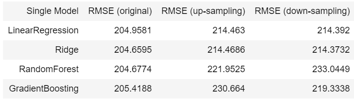
Single Model:

Tandem Model:

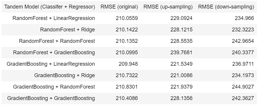
The best model from step 2 is using LinearRegression without any over sampling and down sampling technique. And the best model from step 3 is using RandomForest + LinearRegression without any over sampling and down sampling. Mean squared error for the best model from step 2 and 3 are 214.463 and 210.0559, respectively.

Conclusion

1. For the single regression models, up-sampling and down-sampling technique do not give advantages at all. Actually, they even have higher mean squared error for those four models. Furthermore, we can see that when using resampling methods, mean square error of tree-based models are slightly higher than linear models.
2. I utilised different data preprocessing approaches to encode categorical features, e.g. preprocessing_baseline() and preprocessing_v2(), such as OneHotEncoder() and MeanEncoder(). In baseline preprocessor, I used OneHotEncoder() only to transform the categorical feature. But I found that OneHotEncoder() would produce high sparsity matrix when there’s many categories. Therefore, I subclass a MeanEncoder() in sklearn to deal with high-cardinality categorical features. After the experiment, using MeanEncoder() moderately improves the performance of the models.
3. For the tandem models, I trained the models in two different ways. First, I built a binary classifier, and collected the prediction which is not zero. Next, I fed them into regression model to get the final predicitons. Second, I built a binary classifier as the one before, and after that I selected only non-zero labels in original dataset to feed into regression model. When I done training these two methods, the second one performs better than the first one, so I decided to use the second training method as my pipeline.
4. When comparing single models with tandem models, it can see that single models is better than tandem models whether or not sampling methods are used. Single models’ mean square error are less than tandem models’ by 2.85% in average. However, if we must utilise sampling method to solve imbalanced label problem, it can be seen that over sampling practically outperforms down sampling.