Missionaries and Cannibals Problem

This is actually one of my project when I was in college during my “Mathematical Programming” class. I used R programming language to solve missionaries and cannibals problem with matrix analysis and graph theory.

Introduction

The missionaries and cannibals problem, and the closely related jealous husbands problem, are classic river-crossing logic puzzles. In the missionaries and cannibals problem, three missionaries and three cannibals must cross a river using a boat which can carry at most two people, under the constraint that, for both banks, if there are missionaries present on the bank, they cannot be outnumbered by cannibals (if they were, the cannibals would eat the missionaries). The boat cannot cross the river by itself with no people on board.

Solving

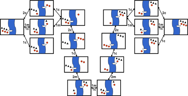
A system for solving the Missionaries and Cannibals problem whereby the current state is represented by a simple vector . The vector’s elements represent the number of missionaries, cannibals, and whether the boat is on the the east side or on the west side, respectively. Suppose the boat and all of the missionaries and cannibals start on the east side, the vector is initialized to . According to the problem, and , therefore, there are different status. However, the nummber of missionaries must be greater than the number of cannibals, and there should always be people on the shoreside while the boat is on that side, so the following states do not exist:

There are only 18 states left, and we use to represent a set of vertexs as following:

We know that everyone departs from east side, that is, the initial vertex is . Suppose 1 missionary and 1 cannibal tend to go from east side to west side, then it should be represented as to , and we will say and are adjacent to each other:

Obviously, the procedure is reversible:

This means the two vertexs has symmetric relation, we then use undirected arrow to connect them. For example, let’s say we make missionaries and cannibals start from , then there will be three possible conditions:

By repeating the above algorithm, we can get an undirected graph.

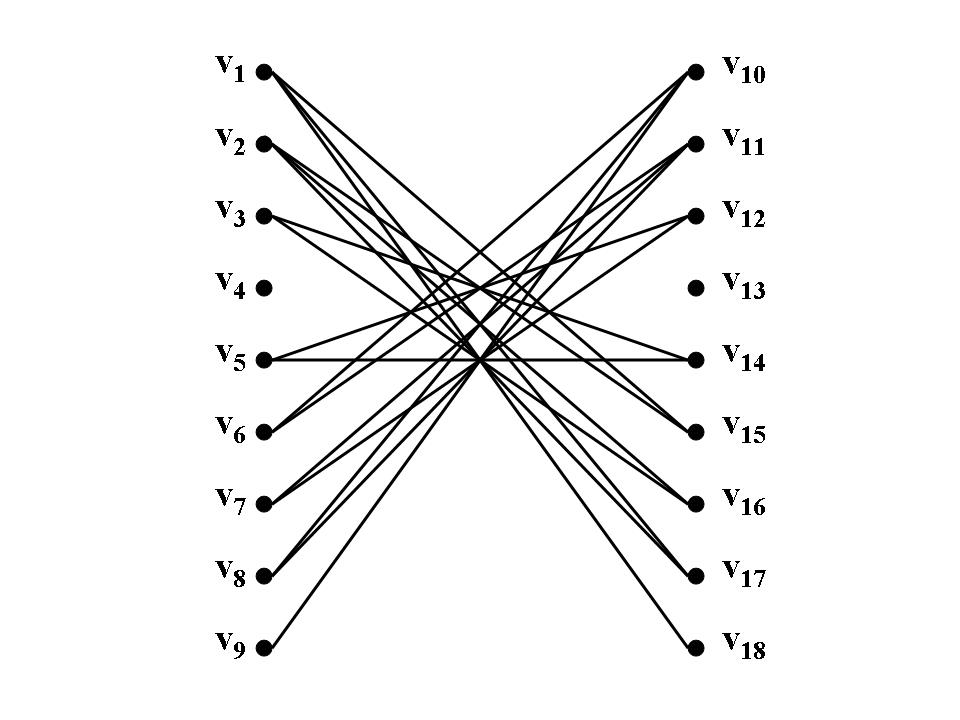
In order to compute this in matrix, I define a adjacency matrix to represent the undirected graph: if and are adjacent to each other, then 1, otherwise 0. Moreover, for every , we let the value be 0, that is, .

where is a symmetric matrix.

From above, we can tell that illustrate and are adjacent to each other. We define the journey starts from to is a series of paths:

If we do not pass through the vertex of repeat visits, which means that are different from each other, then we call it is a path of length . Our goal is to start at and end at , because part of the east side, and belongs to the west side, so the length of the path must be an odd number. For odd numbers , it is not difficult to confirm:

The power of the adjacency matrix , represented as , gives the number of paths of length k between vertices and . (mathematical proof)

This property provides an easy method to find the shortest path: calculated continuously , and until is greater than zero, that is, which means that we have arrived at the destination , but also know the shortest path length is equal to , and the total number of path is equal to .

Computation in R

I define a variable B representing the adjacency matrix mentioned above and build a function to compute the power to a matrix.

B <- matrix(c(
    0, 0, 0, 0, 0, 1, 0, 1, 1, 
    0, 0, 0, 0, 0, 1, 1, 1, 0, 
    0, 0, 0, 0, 1, 0, 1, 0, 0,  
    0, 0, 0, 0, 0, 0, 0, 0, 0,  
    0, 0, 1, 0, 1, 0, 0, 0, 0,  
    1, 1, 0, 0, 0, 0, 0, 0, 0,  
    0, 1, 1, 0, 0, 0, 0, 0, 0,  
    1, 1, 0, 0, 0, 0, 0, 0, 0, 
    1, 0, 0, 0, 0, 0, 0, 0, 0), nrow=9)

power = function(x, n) Reduce(`%*%`, replicate(n, x, simplify=FALSE))

---

For :

power(B, 3)

     [,1] [,2] [,3] [,4] [,5] [,6] [,7] [,8] [,9]
[1,]    0    0    0    0    0    5    2    5    3
[2,]    0    0    0    0    1    5    4    5    2
[3,]    0    0    1    0    3    1    3    1    0
[4,]    0    0    0    0    0    0    0    0    0
[5,]    0    1    3    0    3    0    1    0    0
[6,]    5    5    1    0    0    0    0    0    0
[7,]    2    4    3    0    1    0    0    0    0
[8,]    5    5    1    0    0    0    0    0    0
[9,]    3    2    0    0    0    0    0    0    0

Vertex first visited:

Shortest path length:

Total number of path: 2

---

For :

power(B, 5)

     [,1] [,2] [,3] [,4] [,5] [,6] [,7] [,8] [,9]
[1,]    0    0    0    0    2   25   14   25   13
[2,]    0    0    1    0    6   26   19   26   12
[3,]    0    1    5    0   10    7   11    7    2
[4,]    0    0    0    0    0    0    0    0    0
[5,]    2    6   10    0   10    1    5    1    0
[6,]   25   26    7    0    1    0    0    0    0
[7,]   14   19   11    0    5    0    1    0    0
[8,]   25   26    7    0    1    0    0    0    0
[9,]   13   12    2    0    0    0    0    0    0

Vertex first visited:

Shortest path length:

Total number of path: 2

---

For :

power(B, 7)

     [,1] [,2] [,3] [,4] [,5] [,6] [,7] [,8] [,9]
[1,]    0    0    2    0   18  127   80  127   63
[2,]    0    1    8    0   32  135   96  135   64
[3,]    2    8   21    0   36   41   46   41   16
[4,]    0    0    0    0    0    0    0    0    0
[5,]   18   32   36    0   35    9   22    9    2
[6,]  127  135   41    0    9    0    1    0    0
[7,]   80   96   46    0   22    1    7    1    0
[8,]  127  135   41    0    9    0    1    0    0
[9,]   63   64   16    0    2    0    0    0    0

Vertex first visited:

Shortest path length:

Total number of path: 2

---

For :

power(B, 9)

     [,1] [,2] [,3] [,4] [,5] [,6] [,7] [,8] [,9]
[1,]    0    2   22    0  118  651  432  651  317
[2,]    2   11   49    0  168  700  494  700  334
[3,]   22   49   86    0  139  226  210  226   98
[4,]    0    0    0    0    0    0    0    0    0
[5,]  118  168  139    0  128   60   97   60   20
[6,]  651  700  226    0   60    1   11    1    0
[7,]  432  494  210    0   97   11   38   11    2
[8,]  651  700  226    0   60    1   11    1    0
[9,]  317  334   98    0   20    0    2    0    0

Vertex first visited:

Shortest path length:

Total number of path: 2

---

For :

power(B, 11)

     [,1] [,2] [,3] [,4] [,5] [,6] [,7] [,8] [,9]
[1,]    4   28  164    0  690 3353 2284 3353 1619
[2,]   28   86  277    0  879 3628 2556 3628 1734
[3,]  164  277  360    0  574 1212 1011 1212  550
[4,]    0    0    0    0    0    0    0    0    0
[5,]  690  879  574    0  492  357  442  357  140
[6,] 3353 3628 1212    0  357   15   84   15    2
[7,] 2284 2556 1011    0  442   84  195   84   24
[8,] 3353 3628 1212    0  357   15   84   15    2
[9,] 1619 1734  550    0  140    2   24    2    0

Vertex first visited:

Shortest path length:

Total number of path: 4

---

Therefore all the missionaries and cannibals have crossed the river safely.

Conclusion

As a math major student, it may very well be true that we won’t use some of the more abstract mathematical concepts we learn in school unless we choose to work in specific project. We are taught lots of useless things in math major. However, the underlying skills we developed in mathametics class, such as thinking logically and solving problems, will last a lifetime and help us solve work-related and real-world problems.

References

1. https://ccjou.wordpress.com/2012/08/09/%E6%B8%A1%E6%B2%B3%E5%95%8F%E9%A1%8C/
2. https://stackoverflow.com/questions/3274818/matrix-power-in-r
3. http://page.mi.fu-berlin.de/rote/Papers/pdf/Crossing+the+bridge+at+night.pdf