Demystify Matrix Decomposition

The most important application for decomposition is in data fitting. The following discussion is mostly presented in terms of different methods of decomposition for linear function.

Introduction

The method of least squares is a standard approach in regression analysis to approximate the solution of overdetermined systems (sets of equations in which there are more equations than unknowns) by minimizing the sum of the squares of the residuals made in the results of every single equation. An matrix decomposition is a way of reducing a matrix into its constituent parts. It’s an approach that can specify more complex matrix operation that can be performed on the decomposed matrx rather than on the origin matrix itself. There are various matrix decomposition methods, such as LU decomposition, QR decomposition, SVD decomposition, and Cholesky decomposition, etc.

LU Decomposition

Least Square: Let with , , and . We aim to solve where is the least square estimator. The least squares solution for can obtained using different decomposition methods on .

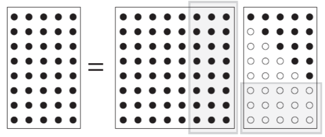
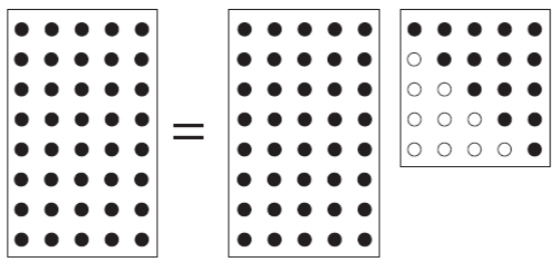
When using LU, we have , decomposing the square matrix into and components. The factors and are triangular matrices. A variation of this decomposition that is numerically more stable to solve in practice is called the PLU decomposition, or the LU decomposition with partial pivoting, where is a so-called permutation matrix, is lower triangular, and is upper triangular. Lower and upper triangular matrices are computationally easier than your typical invertible matrix. The matrix P is easy to deal with as well since it is mostly full of zeros. This video explains how to find the LU decomposition of a square matrix using a shortcut involving the opposite of multipliers used when performing row operations. There is also another posting describe LU and PLU factorisation with some examples.

Pseudocode

Step 1. Start with three candidate matrices:

where is a zeros matrix and is a identity matrix.

Step 2. For , find the row with the largest entry in absolute value on or below the diagonal of the -row and swap rows and in all three matrices, , , and . If this maximum entry is zero, then terminate this loop and indicate that the matrix is singular (invertible).

Step 3. Inside the first loop, create a second for loop, for , calculate the scalar value . Next, add times row onto row in the matrix $U$ and set the entry .

Step 4. Having iterated from , finish by adding the identity matrix onto . These are the , , and matrices of the PLU decomposition of matrix .

class Decomposition:
    """
    References
    ----------
    [1] https://ece.uwaterloo.ca/~dwharder/NumericalAnalysis/04LinearAlgebra/lup/
    [2] https://math.unm.edu/~loring/links/linear_s08/LU.pdf
    [3] https://johnfoster.pge.utexas.edu/numerical-methods-book/LinearAlgebra_LU.html
    """
    def __init__(self):
        pass
    
    def plu(self, A):
        # Step 1. Inittiate three cadidate matrices
        n = A.shape[0]
        P = np.identity(n)
        L = np.identity(n)
        U = A.copy()
        
        PF = np.identity(n)
        LF = np.zeros(shape=(n, n))
        
        # Step 2. Loop over rows find the row with the largest entry in absolute
        # value on or below the diagonal of the i-th row
        for i in range(n-1):
            index = np.argmax(abs(U[i:, i]))
            index = index + i
            if index != i:
                P = np.identity(n)
                P[[index, i], i:n] = P[[i, index], i:n]
                U[[index, i], i:n] = U[[i, index], i:n] 
                PF = np.dot(P, PF)
                LF = np.dot(P, LF)
            L = np.identity(n)
            # Step 3. Calculate the scalar value
            for j in range(i+1, n):
                L[j, i]  = -(U[j, i] / U[i, i])
                LF[j, i] =  (U[j, i] / U[i, i])
            U = np.dot(L, U)
        # Step 4. Add identity matrix onto L
        np.fill_diagonal(LF, 1)
        return PF, LF, U

QR decomposition

In linear algebra, a QR decomposition, also known as a QR factorization or QU factorization is a decomposition of a matrix , either square or rectangular, into a product of an orthogonal matrix and an upper triangular matrix . There are in fact a couple of methods to compute a QR decomposition. These include the the Gram–Schmidt process, Householder transformations, and Givens rotations.

If has linearly independent columns, then it can factored as:

where are orthogonal -vectors (), that is, , if . Moreover, diagonal elements are nonzero ( is nonsingular), and most definitions require , this makes and unique.

Before dive into how to calculate QR factorisation, we should know what problem or application we can tackle with or apply for.

• Linear equations
• Generalised linear regression model
• Singular-value decomposition in the Jacobi-Kogbetliantz approach
• Automatic removal of an object from an image

Algorithms for QR

1. Gram-Schmidt process

• Complexity is flops
• Not recommended in practice (sensitive to rounding errors)

2. Modified Gram-Schmidt process

• Complexity is flops
• Better numerical properties

3. Householder transformations

• Complexity is flops
• Represents as a product of elementary orthogonal matrices
• The most widely used algorithm

Gram-Schmidt Process

The goal of Gram-Schmidt process is to calculate orthogonal basis from original basis , and this can also be represented in summation notation:

A full calculation process can be found in this youtube video presented by Dave.

Matlab code

function [Q, R] = gram_schmidt_qr(A)
    [m, n] = size(A);
    Q = zeros(m, n);
    R = zeros(n, n);
    for j = 1:n
        R(1:j-1, j) = Q(:, 1:j-1)' * A(:, j);
        v = A(:, j) - Q(:, 1:j-1) * R(1:j-1, j);
        R(j, j) = norm(v);
        Q(:, j) = v / R(j, j);
    end;

Python code

class Decomposition:
    def __init__(self):
        pass

    def gram_schmidt_qr(self, A):
        m, n = A.shape
        Q = np.zeros(shape=(m, n))
        R = np.zeros(shape=(n, n))
        for j in range(n):
            v = A[:, j]
            for i in range(j):
                q = Q[:, i]
                R[i, j] = q.dot(v)
                v = v - R[i, j] * q
            Q[:, j] = v / np.linalg.norm(v)
            R[j, j] = np.linalg.norm(v)
        return Q, R

Modified Gram-Schmidt Process

In 1966 John Rice showed by experiments that the two different versions of the Gram–Schmidt orthogonalization, classical (CGS) and modified (MGS) have very different properties when executed in finite precision arithmetic. Only for n = 2 are CGS and MGS numerically equivalent.

Instead of computing the vector as , it is computed as:

where .

Matlab code

function [Q, R] = modified_gram_schmidt_qr(A)
    [m, n] = size(A);
    Q = A;
    R = zeros(n);
    for k = 1:n
        R(k, k) = norm(Q(:, k));
        Q(:, k) = Q(:, k) / R(k, k);
        R(k, k+1:n) = Q(:,k)' * Q(:, k+1:n);
        Q(:, k+1:n) = Q(:, k+1:n) - Q(:, k) * R(k, k+1:n);
    end

Python code

class Decomposition:
    def __init__(self):
        pass

    def modified_gram_schmidt_qr(self, A):
        m, n = A.shape
        Q = np.zeros(shape=(m, n))
        R = np.zeros(shape=(n, n))
        for j in range(0, n):
            R[j, j] = np.sqrt(np.dot(A[:, j], A[:, j]))
            Q[:, j] = A[:, j] / R[j, j]
            for i in range(j+1, n):
                R[j, i] = np.dot(Q[:, j], A[:, i])
                A[:, i] = A[:, i] - R[j, i] * Q[:, j]
        return Q, R

Householder Transformations

Householder transformations are simple orthogonal transformations corresponding to reflection through a plane. Reflection across the plane orthogonal to a unit normal vector can be expressed in matrix form as

In particular, if we take where and then

Let us first verify that this works:

and

so

finally

As a byproduct of this calculation, note that we have

where ; and if we define , we have

where .

Matlab code

function [Q,R] = householder_qr(A)
    [m, n] = size(A);
    Q = eye(m);
    R = A;
    I = eye(n);

    for j = 1:n-1
        x = R(j:n, j);
        v = -sign(x(1)) * norm(x) * eye(n-j+1, 1) - x;
        if norm(v) > 0
            v = v / norm(v);
            P = I;
            P(j:n, j:n) = P(j:n, j:n) - 2*v*v';
            R = P * R;
            Q = Q * P;
        end
    end

Python code

class Decomposition:
    """
    https://stackoverflow.com/a/53493770/15048366
    """
    def __init__(self):
        pass

    def householder_vectorised(self, arr):
        v = arr / (arr[0] + np.copysign(np.linalg.norm(arr), arr[0]))
        v[0] = 1
        tau = 2 / (v.T @ v)
        return v, tau

    def householder_qr(self, A):
        m, n = A.shape
        Q = np.identity(m)
        R = A.copy()

        for j in range(0, n):
            v, tau = self.householder_vectorised(R[j:, j, np.newaxis])
            H = np.identity(m)
            H[j:, j:] -= tau * (v @ v.T)
            R = H @ R
            Q = H @ Q

        Q, R = Q[:n].T, np.triu(R[:n])
        for i in range(n):
            if R[i, i] < 0:
                Q[:, i] *= -1
                R[i, :] *= -1
                
        return Q, R

if :

• Full QR factorisation

  

• Reduced QR factorisation

  

Linear Function

After decomposing matrix , you can write a function in python to solve a system

using LU decomposition and QR decomposition. Your function should take and as input and return .

Function should include the following:

• Check that is not a singular matrix, that is, is invertible.
• Invert using different decomposition methods and solve
• Return .

class Decomposition:
    
    def plu(self, A):
        n = A.shape[0]
        P = np.identity(n)
        L = np.identity(n)
        U = A.copy()
        
        PF = np.identity(n)
        LF = np.zeros(shape=(n, n))
        
        # Loop over rows
        for i in range(n-1):
            index = np.argmax(abs(U[i:, i]))
            index = index + i
            if index != i:
                P = np.identity(n)
                P[[index, i], i:n] = P[[i, index], i:n]
                U[[index, i], i:n] = U[[i, index], i:n] 
                PF = np.dot(P, PF)
                LF = np.dot(P, LF)
            L = np.identity(n)
            for j in range(i+1, n):
                L[j, i]  = -(U[j, i] / U[i, i])
                LF[j, i] =  (U[j, i] / U[i, i])
            U = np.dot(L, U)
        np.fill_diagonal(LF, 1)
        return PF, LF, U
    
    def gram_schmidt_qr(self, A):
        m, n = A.shape
        Q = np.zeros(shape=(m, n), dtype='float64')
        R = np.zeros(shape=(n, n), dtype='float64')
        for j in range(n):
            v = A[:, j]
            for i in range(j):
                q = Q[:, i]
                R[i, j] = q.dot(v)
                v = v - R[i, j] * q
            Q[:, j] = v / np.linalg.norm(v)
            R[j, j] = np.linalg.norm(v)
        return Q, R
    
    def modified_gram_schmidt_qr(self, A):
        n = A.shape[1]
        Q = np.array(A, dtype='float64')
        R = np.zeros((n, n), dtype='float64')
        for k in range(n):
            a_k = Q[:, k]
            R[k,k] = np.linalg.norm(a_k)
            a_k /= R[k, k]
            for i in range(k+1, n):
                a_i = Q[:, i]
                R[k,i] = np.transpose(a_k) @ a_i
                a_i -= R[k, i] * a_k
        return Q, R
    
    def householder_vectorised(self, arr):
        v = arr / (arr[0] + np.copysign(np.linalg.norm(arr), arr[0]))
        v[0] = 1
        tau = 2 / (v.T @ v)
        return v, tau

    def householder_qr(self, A):
        m, n = A.shape
        Q = np.identity(m)
        R = A.copy()

        for j in range(0, n):
            v, tau = self.householder_vectorised(R[j:, j, np.newaxis])
            H = np.identity(m)
            H[j:, j:] -= tau * (v @ v.T)
            R = H @ R
            Q = H @ Q

        Q, R = Q[:n].T, np.triu(R[:n])
        for i in range(n):
            if R[i, i] < 0:
                Q[:, i] *= -1
                R[i, :] *= -1
                
        return Q, R

def linear_function_solver(A, b, method="LU"):
    det = ChioDeterminants().calculate(A)
    factoriser = Decomposition()
    if det == 0:
        print("Matrix is singular!")
        return
    if method == "LU":
        P, L, U = factoriser.plu(A)
        z_1 = P.T @ b
        z_2 = np.linalg.inv(L) @ z_1
        x = np.linalg.inv(U) @ z_2
        return x
    elif method == "CGS":
        Q, R = factoriser.gram_schmidt_qr(A)
        x = np.linalg.inv(R) @ Q.T @ b
        return x
    elif method == "MGS":
        Q, R = factoriser.modified_gram_schmidt_qr(A)
        x = np.linalg.inv(R) @ Q.T @ b
        return x
    elif method == "HHT":
        Q, R = factoriser.householder_qr(A)
        x = np.linalg.inv(R) @ Q.T @ b
        return x

Let’s check on four different approachs.

A = np.array([
    [8, 6, 4, 1], 
    [1, 4, 5, 1], 
    [7, 4, 2, 5], 
    [1, 4, 2, 6]])
b = np.array([20, 12, 23, 19])

print("NP:  ", np.linalg.solve(A, b))
print("LU:  ", linear_function_solver(A, b, method="LU"))
print("CGS: ", linear_function_solver(A, b, method="CGS"))
print("MGS: ", linear_function_solver(A, b, method="MGS"))
print("HHT: ", linear_function_solver(A, b, method="HHT"))

---

NP:   [1. 1. 1. 2.]
LU:   [1. 1. 1. 2.]
CGS:  [1. 1. 1. 2.]
MGS:  [1. 1. 1. 2.]
HHT:  [1. 1. 1. 2.]

Conclusion

In this article, I implement different matrix decomposition methods, named LU decomposition and QR decomposition (Gram-Schmidt process, Modified Gram-Schmidt process, Householder transformations). In the future, I may apply matrix decomposition algorithm to neural networks. I hope it will be much more efficient than the regularisers methods.

References

1. https://ece.uwaterloo.ca/~dwharder/NumericalAnalysis/04LinearAlgebra/lup/
2. https://math.unm.edu/~loring/links/linear_s08/LU.pdf
3. https://johnfoster.pge.utexas.edu/numerical-methods-book/
4. https://web.cs.ucdavis.edu/~bai/publications/andersonbaidongarra92.pdf
5. https://deepai.org/machine-learning-glossary-and-terms/qr-decomposition
6. https://en.wikipedia.org/wiki/Matrix_decomposition
7. http://homepages.math.uic.edu/~jan/mcs507f13/
8. https://www.cis.upenn.edu/~cis610/Gram-Schmidt-Bjorck.pdf
9. https://wikivisually.com/wiki/Gram%E2%80%93Schmidt_process
10. https://rpubs.com/aaronsc32/qr-decomposition-householder
11. https://www.cs.cornell.edu/~bindel/class/cs6210-f09/lec18.pdf
12. https://homel.vsb.cz/~dom033/predmety/parisLA/05_orthogonalization.pdf
13. https://core.ac.uk/download/pdf/82066579.pdf