Speech

Publish Date: 2021-02-05

Word Count: 3.4k

Read Times: 21 Min

Read Count:

Visualizing sound is kind of a trippy concept. There are some mesmerizing ways to do that, and also more mathematical ones, which I will explore both in this article.

Introduction

I wrote an [article] about lyrics-based song genre classifier before. I was wondering whether using the audio-based data will improve the performance. For this reason, this work takes a closer look at expoiting audio-based approach to build a multi-class classifier.

Audio Processing

Let’s take one song for instance,

Librosa

librosa is a python package for music and audio analysis. It provides the building blocks necessary to create music information retrieval systems. Let’s load the audio file we want to process first.

signal, sr = librosa.load("Halo.mp3")

Great, a wonderful song, isn’t it? Then how does the sound look like in a graph?

Waveform

We can now take a look at its waveform. The waveform of a signal is the shape of its graph as a function of time, independent of its time and magnitude scales and of any displacement in time. Here is a interesting animation of waveform written by Josh Comeau.

plt.rcParams["figure.figsize"] = 15, 6
librosa.display.waveplot(signal, sr=sr, alpha=0.5)
plt.xlabel("Time")
plt.ylabel("Amplitude")
plt.show()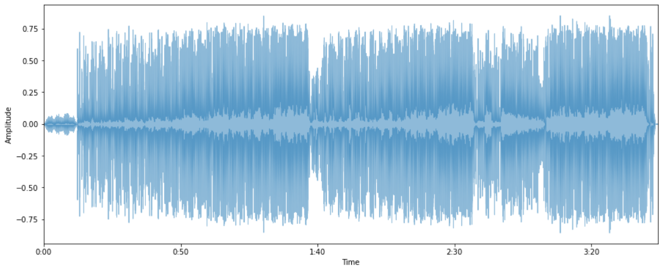

Sampling Rate

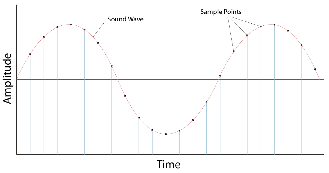
When we use librosa.load() we can set a parameter called “sr”, which stands for “sampling rate”, but what exactly does this mean? In audio production, a sampling rate defines how many times per second a sound is sampled, that is, the number of amplitude that can be recorded per second. For example, the sampling rate is 1khz, which means that the amplitude of 1000 waves can be recorded in one second.

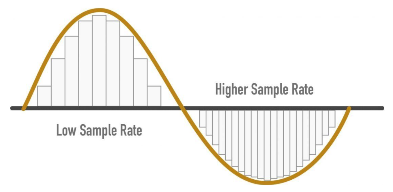
The default sampling rate used by Librosa is 22050, but you can pass in almost any sampling rate you like. Further, the higher sample rate technically leads to more measurements per second and a closer recreation of the original audio, so 48 kHz is often used in “professional audio” contexts more than music contexts.

We can also indicate that sampling rate (Hz) is the inverse of the period . Look at the figure below in detail, the higher the sample rate, the less the sampling error.

How many samples are necessary to ensure we are preserving the information contained in the signal? If the signal contains high frequency components, we will need to sample at a higher rate to avoid losing information that is in the signal. In general, to preserve the full information in the signal, it is necessary to sample at twice the maximum frequency of the signal. This is known as the Nyquist rate. The Sampling Theorem states that a signal can be exactly reproduced if it is sampled at a frequency F, where F is greater than twice the maximum frequency in the signal.

What happens if we sample the signal at a frequency that is lower that the Nyquist rate? When the signal is converted back into a continuous time signal, it will exhibit a phenomenon called ‘aliasing’. Aliasing is the presence of unwanted components in the reconstructed signal. These components were not present when the original signal was sampled. In addition, some of the frequencies in the original signal may be lost in the reconstructed signal. Aliasing occurs because signal frequencies can overlap if the sampling frequency is too low.

Frames

Perceivable audio to chunk.
Power of 2 # of samples.
Typical values: 256 ~ 8192.

Formula for duration of a frame:

where is duration of a frame, is sample rate, and is the frame size.

Spectral Leakage

Processed signal isn’t an integer number of periods.
Endpoints are discontinuous.
Discontinuous appear as high-frequency components not present in the original signal.

Windowing

Apply windowing function to each frame.
Eliminates samples t both ends of a frame.
Generates a periodic signal.

Hann Window

This function is a member of both the cosine-sum and power-of-sine families. The end points of the Hann window just touch zero.

At both endpoints will touch zero, which is a problem losing a signal. The solution to this is to overlap the frames.

Bit Depth & Bit Rate

Analog audio is a continuous wave, with an effectively infinite number of possible amplitude values. However, to measure this wave in digital audio, we need to define the wave’s amplitude as a finite value each time we sample it.

To illustrate bit depth, suppose you want to draw a picture of a sunset, but you only have 16 crayons. In real-life, sunsets come in a variety of colors, from dazzling yellows and oranges to faint reds and purples. If there were only 16 crayons, then it would be impossible to really draw all these different colors. What If you have 32 crayons, you can then use twice as many colors, although the picture still doesn’t look realistic. Thereupon, if you continue to add more crayons, you can definitely draw better.

The bit depth determines the number of possible amplitude values we can record for each sample. The most common bit depths are 16-bit, 24-bit, and 32-bit. Each is a binary term, representing a number of possible values. Systems of higher bit depths are able to express more possible values.

The bit rate of a file tells us how many bits of data are processed every second. Bit rates are usually measured in kilobits per second (kbps). To calculate the bit rate, we can use the following formula:

A typical, uncompressed high-quality audio file has a sample rate of 44,100 samples per second, a bit depth of 16 bits per sample and 2 channels of stereo audio. The bit rate for this file would be: 44100 samples per second × 16 bits per sample × 2 channels = 1411200 bits per second (or 1411.2 kbps).

To sum up, we can know that the higher the bit rate, the faster the data transfer speed. With a firmer understanding of sample rate and bit depth, let’s dive in next topic - spectrum.

Spectrum

Before we talk about the spectrum, we need to understand the sound waves first.

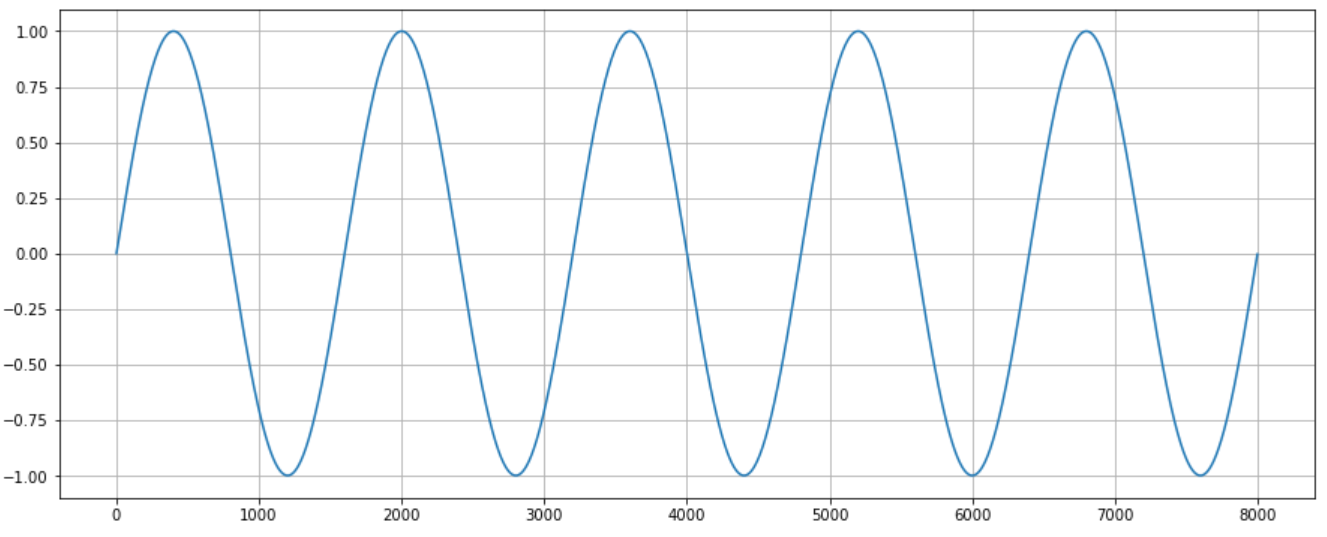
Amplitude: the greater the amplitude, the louder the volume of the sound, and vice versa the lower the volume.
Cycle: from position 0, to the peak, then to the trough, and finally back to 0, this is called a cycle.
Frequency: frequency refers to how many cycles per second, the higher the frequency, the higher the pitch.
Phase: indicates the position of the waveform in the cycle, measured in degrees.
Wavelength: denotes the distance between two points with the same phase degree. The longer the wavelength, the lower the frequency, the shorter the wavelength, the higher the frequency.

So what is a Spectrum? A spectrum displays the different frequencies present in a sound.

fft = np.fft.fft(signal)
magnitude = np.absolute(fft)
frequency = np.linspace(0, sr, len(magnitude))
left_frequency = frequency[:int(len(frequency)/2)]
left_magnitude = magnitude[:int(len(magnitude)/2)]

plt.plot(left_frequency, left_magnitude, color="tab:blue")
plt.xlabel("Frequency")
plt.ylabel("Magnitude")
plt.grid()
plt.show()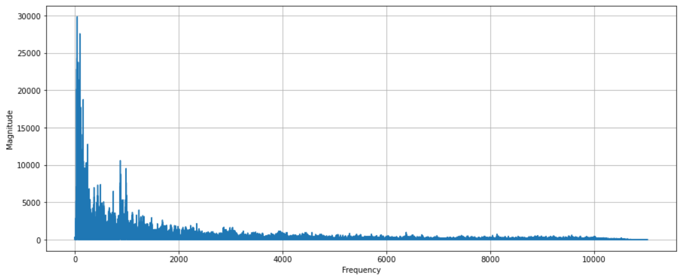

I use np.fft.fft to perform Discrete Fourier Transform (DFT) with the efficient Fast Fourier Transform (FFT) algorithm. Fourier Transform is another mathematical representation of sound. Fourier Transform is a function that gets a signal in the time domain as input, and outputs its decomposition into frequencies.

The Fourier Transform is one of deepest insights ever made. Unfortunately, the meaning is buried within dense equations:

Rather than jumping into the symbols, let’s experience the key idea firsthand. Here’s a plain-English metaphor from this article:

What does the Fourier Transform do? Given a smoothie, it finds the recipe.
How? Run the smoothie through filters to extract each ingredient.
Why? Recipes are easier to analyze, compare, and modify than the smoothie itself.
How do we get the smoothie back? Blend the ingredients.

The Fourier Transform changes our perspective from consumer to producer, turning What do I have? into How was it made? In other words: given a smoothie, let’s find the recipe. In the process of filtration, the components and proportions do not change, so we can reverse the formula through this transformation, which is the meaning of the filter.

We can now derive the Discrete Fourier Transform from the continuous version of the Fourier series development.

Let’s implement discrete fourier transform in python.

def dft(x):
    x = np.asarray(x, dtype=float)
    N = x.shape[0]
    cos = np.zeros_like(x)
    sin = np.zeros_like(x)
    X = []
    for k in range(N):
        real, image = 0, 0
        for n in range(N):
            real += x[n] * math.cos(2 * math.pi * k * n / N)
            image += x[n] * math.sin(2 * math.pi * k * n / N)
        X.append(complex(real, image))
    return np.array(X)

Check whether it is correct.

x = np.random.rand(1000, )
((fft(x) - np.fft.fft(x)) < 1e-10).all()

True

Intuition

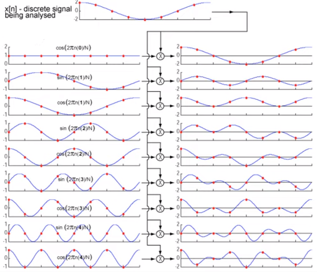
Decompose a complex sound into its frequency components.
Convert time domain to frequency domain.
Compare signal with sinusoids of various frequencies.
For each frequency we get a magnitude and a phase.
High magnitude indicates high similarity bwtween the signal and a sinunoid.

Reconstruct the signal

Superimpose sinusoids
Weight them bu the relative magnitude
Use relative phase
Original signal and FT have same information

Inverse Fourier Transform

Additive synthesis (waveform -> spectrum -> waveform)

Spectrogram

Short-time Fourier transform (STFT) is a sequence of Fourier transforms of a windowed signal. STFT provides the time-localized frequency information for situations in which frequency components of a signal vary over time, whereas the standard Fourier transform provides the frequency information averaged over the entire signal time interval. In this work, I use STFT to obtain sprectrogram.

A spectrogram is a visual way of representing the signal strength, or “loudness”, of a signal over time at various frequencies present in a particular waveform. Not only can one see whether there is more or less energy at, but one can also see how energy levels vary over time.

n_fft = 2048
hop_length = 512

stft = librosa.core.stft(signal, n_fft=n_fft, hop_length=hop_length)
spectrogram = np.abs(stft)
log_spectrogram = librosa.amplitude_to_db(spectrogram)

librosa.display.specshow(log_spectrogram, sr=sr, hop_length=hop_length)
plt.xlabel("Time")
plt.ylabel("Frequency")
plt.colorbar()
plt.show()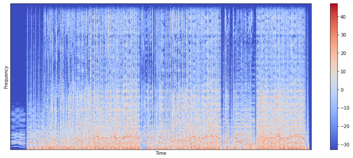

Mel-frequency Cepstrum Coefficients (MFCC)

Mel-frequency cepstral coefficients (MFCCs) are coefficients that collectively make up an MFC. They are derived from a type of cepstral representation of the audio clip (a nonlinear “spectrum-of-a-spectrum”). The advantage of MFCC is that it is good in error reduction and able to produce a robust feature when the signal is affected by noise.

mfcc = librosa.feature.mfcc(signal, n_fft=n_fft, hop_length=hop_length, n_mfcc=13)
librosa.display.specshow(mfcc, sr=sr, hop_length=hop_length)
plt.xlabel("Time")
plt.ylabel("MFCC")
plt.colorbar()
plt.show()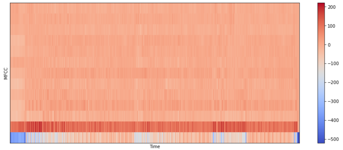

Time-domain Features

Amplitude envelope (AE)
Root-mean-square energy (RMS)
Zero-crossing rate (ZCR)

Amplitude envelope

Max value of all samples in a frame:

Gives rough idea of loudness
Sensitive to outliers
Onset detection, music genre classification

def amplitude_envelope(signal, frame_length, hop_length):
    amplitude_envelope = []
    for i in range(0, len(signal), hop_length):
        current_frame_amplitude_envelope = max(signal[i:i+frame_length])
        amplitude_envelope.append(current_frame_amplitude_envelope)
    return np.array(amplitude_envelope)

FRAME_LENGTH = 1024
HOP_LENGTH = 512

ae_blank_space = amplitude_envelope(blank_space, FRAME_LENGTH, HOP_LENGTH)
frames = range(0, ae_blank_space.size)
t_interval = librosa.frames_to_time(frames, hop_length=HOP_LENGTH)

librosa.display.waveplot(blank_space, alpha=0.5)
plt.plot(t_interval, ae_blank_space, color="tab:red")
plt.title("Taylor Swift Blank Space Amplitude Envelope")
plt.ylim((-1, 1))
plt.show()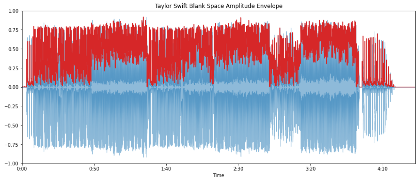

Root-mean-square energy

RMS of all samples in a frame:

Indicator of loudness.
Less sensitive to outliers than AE.
Audio segmentation, music genre classification

FRAME_LENGTH = 1024
HOP_LENGTH = 512

rms_blank_space = librosa.feature.rms(blank_space, frame_length=FRAME_LENGTH, hop_length=HOP_LENGTH)[0]
frames = range(0, rms_blank_space.size)
t_interval = librosa.frames_to_time(frames, hop_length=HOP_LENGTH)

librosa.display.waveplot(blank_space, alpha=0.5)
plt.plot(t_interval, rms_blank_space, color="tab:red")
plt.title("Taylor Swift Blank Space Root-mean-square energy")
plt.ylim((-1, 1))
plt.show()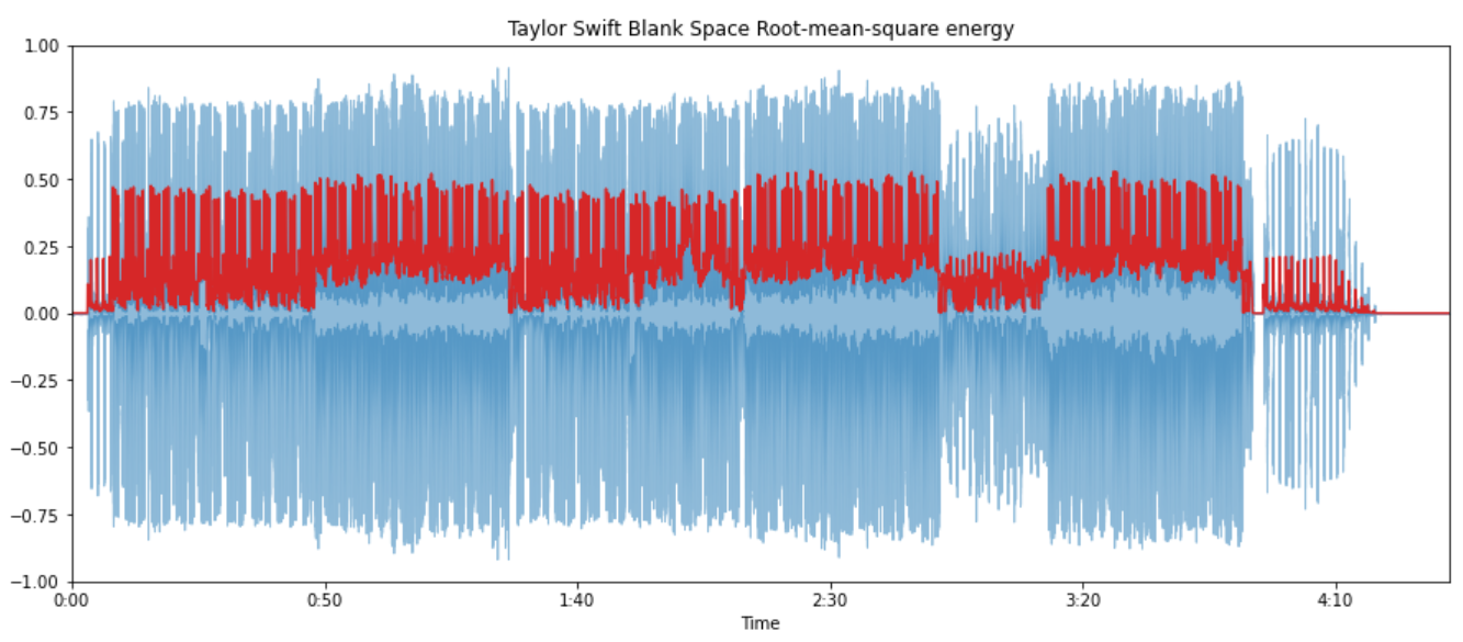

We can also build the function by ourselves.

def root_mean_square(signal, frame_length, hop_length):
    rms = []
    for i in range(0, len(signal), hop_length):
        current_frame_rms = np.sqrt(np.sum(np.square(signal[i:i+frame_length])) / frame_length)
        rms.append(current_frame_rms)
    return np.array(rms)

rms_blank_space_from_scratch = root_mean_square(blank_space, FRAME_LENGTH, HOP_LENGTH)
frames = range(0, rms_blank_space_from_scratch.size)
t_interval = librosa.frames_to_time(frames, hop_length=HOP_LENGTH)

librosa.display.waveplot(blank_space, alpha=0.5)
plt.plot(t_interval, rms_blank_space_from_scratch, color="tab:red")
plt.title("Taylor Swift Blank Space Root-mean-square energy from scratch")
plt.ylim((-1, 1))
plt.show()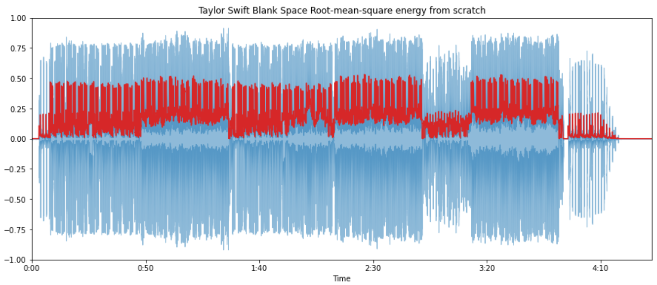

Zero-crossing rate

Number of times a signal crosses the horizontal axis:

Recognition of percussive vs pitched sounds
Monophonic pitch estimation
Voice / Unvoiced decision for speech signals

zrc_blank_space = librosa.feature.zero_crossing_rate(blank_space, frame_length=FRAME_LENGTH, hop_length=HOP_LENGTH)[0]
frames = range(0, zrc_blank_space.size)
t_interval = librosa.frames_to_time(frames, hop_length=HOP_LENGTH)

plt.plot(t_interval, zrc_blank_space*FRAME_LENGTH, color="tab:red")
plt.title("Taylor Swift Blank Zero-crossing rate")
plt.ylim((-50, 600))
plt.show()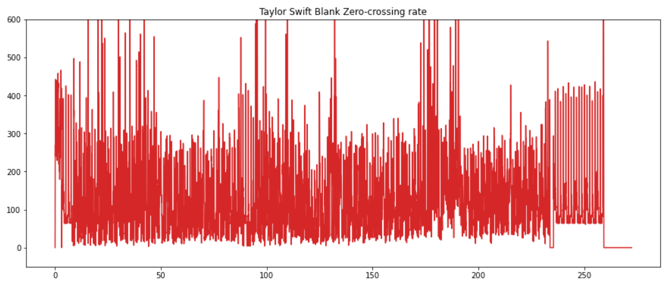

Prepare Data

import os
import json
import math

DATASETPATH = "mp3"
JSONPATH = "data.json"

def save_mfcc(dataset_path, json_path, sr=22050, duration=30, n_mfcc=13, n_fft=2048, hop_length=512, num_segment=5):
    data = {
        "mapping": [], 
        "mfcc": [], 
        "labels": []
    }
    samples_per_track = sr * duration
    num_samples_per_segment = int(samples_per_track / num_segment)
    expected_num_mfcc_vectors_per_segment = math.ceil(num_samples_per_segment / hop_length)
    
    # Loop through all the genre folders
    for i, (dirpath, dirnames, filenames) in enumerate(os.walk(dataset_path)):
        if dirpath is not dataset_path:
            # Save semantic labels
            dirpath_components = dirpath.split("/")
            semantic_label = dirpath_components[-1]
            data["mapping"].append(semantic_label)
            print(f"\nProcessing {semantic_label}")
            
            # Process files for a specific genres
            for f in filenames:
                file_path = os.path.join(dirpath, f)
                signal, sr = librosa.load(file_path, sr=sr)
                
                # Process segments extracting mfcc and store data
                for s in range(num_segment):
                    start_sample = num_samples_per_segment * s
                    finish_sample = start_sample + num_samples_per_segment
                    mfcc = librosa.feature.mfcc(signal[start_sample:finish_sample], 
                                                sr=sr, 
                                                n_mfcc=13, 
                                                n_fft=2048, 
                                                hop_length=512)
                    mfcc = mfcc.T
                    
                    # Store mfcc for segment if it has the expected length
                    if len(mfcc) == expected_num_mfcc_vectors_per_segment:
                        data["mfcc"].append(mfcc.tolist())
                        data["labels"].append(i-1)
                        print(f"{file_path} | segments: {s+1}")
    
    # Save data to a json file
    with open(json_path, "w") as fp:
        json.dump(data, fp, indent=4)

def load_data(json_path):
    with open(json_path, "r") as fp:
        data = json.load(fp)
        
    features = np.array(data["mfcc"])
    targets = np.array(data["labels"])
    
    return features, targets

save_mfcc(DATASETPATH, JSONPATH)
features, targets = load_data(JSONPATH)

Split the data into training dataset and validation dataset.

from sklearn.model_selection import train_test_split

X_trainvalid, X_test, y_trainvalid, y_test = train_test_split(features, targets, test_size=0.1, stratify=targets)
X_train, X_valid, y_train, y_valid = train_test_split(X_trainvalid, y_trainvalid, test_size=0.125, stratify=y_trainvalid)

Modeling

Load the libraries.

import tez
import torch
import torch.nn as nn
from sklearn import metrics, model_selection, preprocessing
from tez.callbacks import EarlyStopping
from tez import enums
from tez.utils import AverageMeter
from torch.utils.data import Dataset
from torch.nn import functional as F
from collections import defaultdict
from tqdm import tqdm

Create Dataset() class from PyTorch.

class SongGenreDataset(Dataset):
    
    def __init__(self, features, targets):
        self.features = features
        self.targets = targets

    def __len__(self):
        return len(self.features)

    def __getitem__(self, idx):
        target = self.targets[idx]
        target = np.array(target)
        target = target.astype(np.float64)
        feature = self.features[idx]
        feature = np.array([feature])
        feature = feature.astype(np.float64)
        feature = np.expand_dims(feature, axis=1)
        sample = {
            'feature': torch.from_numpy(feature).float(), 
            'target': torch.from_numpy(target)}
        return sample

train_dataset = SongGenreDataset(X_train, y_train)
valid_dataset = SongGenreDataset(X_valid, y_valid)
test_dataset = SongGenreDataset(X_test, y_test)

Create a simple MLP model.

class SongGenreMLPClassifier(tez.Model):
    def __init__(self, num_classes):
        super().__init__()
        self.dropout = nn.Dropout(0.1)
        self.fc1 = nn.Linear(259*13, 128)
        self.out = nn.Linear(128, num_classes)
        self.step_scheduler_after = "epoch"
        self.num_classes = num_classes
        self.history = defaultdict(list)

    def monitor_metrics(self, outputs, targets):
        if targets is None:
            return {}
        outputs = torch.argmax(outputs, dim=1).cpu().detach().numpy()
        targets = targets.cpu().detach().numpy()
        accuracy = metrics.accuracy_score(targets, outputs)
        return {"accuracy": accuracy}

    def fetch_optimizer(self):
        opt = torch.optim.Adam(self.parameters(), lr=3e-4)
        return opt

    def fetch_scheduler(self):
        sch = torch.optim.lr_scheduler.CosineAnnealingWarmRestarts(
            self.optimizer, T_0=10, T_mult=1, eta_min=1e-6, last_epoch=-1
        )
        return sch

    def train_one_epoch(self, data_loader):
        self.train()
        self.model_state = enums.ModelState.TRAIN
        losses = AverageMeter()
        tk0 = tqdm(data_loader, total=len(data_loader))
        for b_idx, data in enumerate(tk0):
            self.train_state = enums.TrainingState.TRAIN_STEP_START
            loss, metrics = self.train_one_step(data)
            self.train_state = enums.TrainingState.TRAIN_STEP_END
            losses.update(loss.item(), data_loader.batch_size)
            if b_idx == 0:
                metrics_meter = {k: AverageMeter() for k in metrics}
            monitor = {}
            for m_m in metrics_meter:
                metrics_meter[m_m].update(metrics[m_m], data_loader.batch_size)
                monitor[m_m] = metrics_meter[m_m].avg
            self.current_train_step += 1
            tk0.set_postfix(loss=losses.avg, stage="train", **monitor)
        tk0.close()
        self.update_metrics(losses=losses, monitor=monitor)
        for k, v in monitor.items():
            self.history[f"train_{k}"].append(v)
        self.history["train_loss"].append(losses.avg)
        return losses.avg

    def validate_one_epoch(self, data_loader):
        self.eval()
        self.model_state = enums.ModelState.VALID
        losses = AverageMeter()
        tk0 = tqdm(data_loader, total=len(data_loader))
        for b_idx, data in enumerate(tk0):
            self.train_state = enums.TrainingState.VALID_STEP_START
            with torch.no_grad():
                loss, metrics = self.validate_one_step(data)
            self.train_state = enums.TrainingState.VALID_STEP_END
            losses.update(loss.item(), data_loader.batch_size)
            if b_idx == 0:
                metrics_meter = {k: AverageMeter() for k in metrics}
            monitor = {}
            for m_m in metrics_meter:
                metrics_meter[m_m].update(metrics[m_m], data_loader.batch_size)
                monitor[m_m] = metrics_meter[m_m].avg
            tk0.set_postfix(loss=losses.avg, stage="valid", **monitor)
            self.current_valid_step += 1
        tk0.close()
        self.update_metrics(losses=losses, monitor=monitor)
        for k, v in monitor.items():
            self.history[f"valid_{k}"].append(v)
        self.history["valid_loss"].append(losses.avg)
        return losses.avg
    
    def forward(self, feature, target=None):
        target = target.long().to(self.device)
        x = feature.reshape(feature.shape[0], -1)
        x = F.relu(self.fc1(x))
        outputs = self.out(self.dropout(x))
        outputs = outputs.float().to(self.device)

        if target is not None:
            loss = nn.CrossEntropyLoss()(outputs, target)
            metrics = self.monitor_metrics(outputs, target)
            return outputs, loss, metrics
        
        return outputs, None, None
    
    def score(self, test_dataset, n_jobs=0):
        
        def softmax(x):
            return np.exp(x) / np.sum(np.exp(x), axis=0)
        
        prediction = self.predict(test_dataset, n_jobs=n_jobs)
        prediction = list(prediction)
        prediction = softmax(np.vstack(prediction))
        prediction = np.argmax(prediction, axis=1)
        groud_truth = test_dataset[:]["target"].detach().numpy().astype(np.int64)
        return metrics.accuracy_score(prediction, groud_truth)
    
    def plot_history(self):
        from matplotlib.ticker import MaxNLocator
        
        train_loss, valid_loss = self.history["train_loss"], self.history["valid_loss"]
        train_accuracy, valid_accuracy = self.history["train_accuracy"], self.history["valid_accuracy"]

        plt.rcParams["figure.figsize"] = 15, 6
        ax1 = plt.subplot(2, 1, 1)
        ax1.plot(range(1, len(train_loss)+1), train_loss, color="tab:blue", label="train")
        ax1.plot(range(1, len(valid_loss)+1), valid_loss, color="tab:orange", label="valid")
        ax1.xaxis.set_major_locator(MaxNLocator(integer=True))
        ax1.title.set_text('Loss')
        ax1.grid()
        ax2 = plt.subplot(2, 1, 2)
        ax2.plot(range(1, len(train_accuracy)+1), train_accuracy, color="tab:blue", label="train")
        ax2.plot(range(1, len(valid_accuracy)+1), valid_accuracy, color="tab:orange", label="valid")
        ax2.xaxis.set_major_locator(MaxNLocator(integer=True))
        ax2.title.set_text('Accuracy')
        ax2.grid()
        plt.tight_layout()
        plt.show()

Start training!

model = SongGenreMLPClassifier(num_classes=3)
MODEL_PATH = "./models/"
MODEL_NAME = "SongGenreMLPClassifier"
es = EarlyStopping(
    monitor="valid_loss",
    model_path=os.path.join(MODEL_PATH, MODEL_NAME + ".bin"),
    patience=15,
    mode="min",
)

model.fit(
    train_dataset,
    valid_dataset=valid_dataset,
    train_bs=16,
    valid_bs=16,
    device="cuda",
    epochs=10, 
    fp16=True, 
    callbacks=[es], 
    n_jobs=0
)

model.plot_history()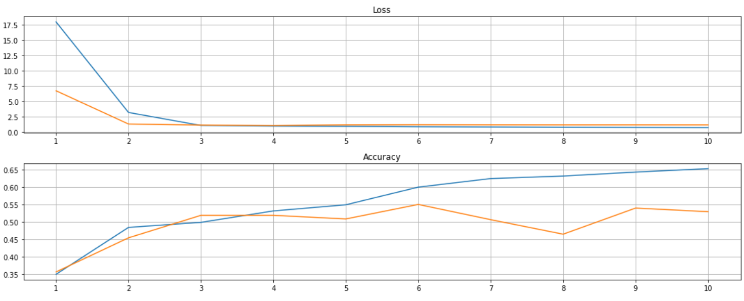

Conclusion

In the end, we got a accuracy score of 50.7% on the test dataset. For your information, I only utilise 150 songs, which is not a large amount of data, but it achieves a higher score than most of the lyrics-based models (this article I wrote before). In the future, I will investigate more different models to improve the performance for the audio-based classifier! Stay tuned!

References

Yang Wang

https://penguinwang96825.github.io/Yang-Tech-Blog/Yang-Tech-Blog/2021/02/05/2021-02-05-audio-based-song-genre-classification/

All articles in this blog are used except for special statements CC BY 4.0 reprint polocy. If reproduced, please indicate source Yang Wang !

Python PyTorch Librosa Speech

SSH into Google Colab

Sometimes the code I write may not work in my local machine, however, it works in Google Colab. So, I wanna connect to Google Colab terminal using SSH.

2021-02-06 Script

Colab SSH

Demystify Matrix Decomposition

The most important application for decomposition is in data fitting. The following discussion is mostly presented in terms of different methods of decomposition for linear function.

2021-01-29 Mathematics

Python MATLAB Linear Algebra

Audio-based Song Genre Classification

Introduction

Audio Processing

Librosa

Waveform

Sampling Rate

Frames

Spectral Leakage

Windowing

Hann Window

Bit Depth & Bit Rate

Spectrum

Intuition

Reconstruct the signal

Inverse Fourier Transform

Spectrogram

Mel-frequency Cepstrum Coefficients (MFCC)

Time-domain Features

Amplitude envelope

Root-mean-square energy

Zero-crossing rate

Prepare Data

Modeling

Conclusion

References