In Data Science interviews, one of the frequently asked questions is What is P-Value?. It’s hard to grasp the concept behind p-value. To understand p-value, you need to understand some background and context behind it. So, let’s start with the basics. When you conduct a piece of quantitative research (such as ML), you are inevitably attempting to answer a research question or hypothesis that you have set. One method of evaluating this research question is via a process called hypothesis testing.
Introduction
In statistics, the p-value is the probability of obtaining results at least as extreme as the observed results of a statistical hypothesis test, assuming that the null hypothesis is correct. In this article, I will explain the concept and the calculation of the p-value in a simple setting.
Hypothesis Testing
P-value is used in hypothesis testing process and its value is used in making decision. Let’s say we have two opposing statements, one is called null hypothesis (denoted as H0), and the other is called alternative hypothesis (denoted as H1). A null hypothesis is a type of conjecture proposes that there’s no difference between certain characteristics of a population (generally about population value being equal to something), and an alternative hypothesis proposed that there’s a difference.
Let’s take an simple example first. We assume that, we want to see if the machine learning average score of CSSLP students is equal to 60, that is, the population mean
The idea here is that we will take a random sample from this population (all CSSLP students), examine the sample and decide whether the samples support our null hypothesis or the alternative hypothesis. So the logic of hypothesis testing indicates that if null hypothesis is true, then the sample mean (suppose you take a random sample) and calculate the sample mean under the null hypothesis, the sample mean should be close to 60, because sample mean and population mean are expected to be close. However, if sample mean is significantly higher than 60, then we will reject null hypothesis and establish the alternative.
Let’s suppose that we took a random sample of 36 CSSLP students from population and calculate the sample mean, and let’s suppose the sample mean is 62 (
Now the question is our
Since
Below is the typical graph of z-scores.
import numpy as np
import matplotlib.pyplot as plt
import scipy.stats as st

plt.figure(figsize=(15, 6))
plt.plot(np.linspace(-4, 4, 100), st.norm.pdf(np.linspace(-4, 4, 100)))
plt.grid()
plt.show()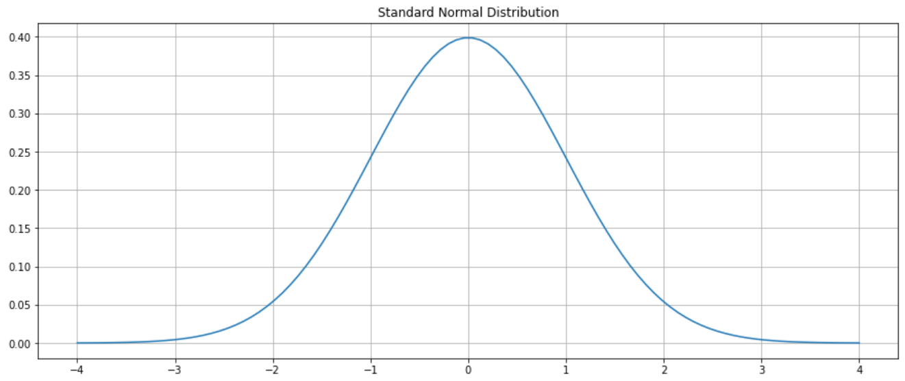
We want to calculate the area under the standard normal curve to the right of 3. This can denoted with the equation below.
from scipy.integrate import quad

def normal_distribution_pdf(x):
    constant = 1.0 / np.sqrt(2*np.pi)
    return(constant * np.exp((-x**2)/2.0))

percentile, _ = quad(normal_distribution_pdf, 3.0, np.Inf)
We can now get the percentile of 0.13%. This probability is called the p-value. To sum up, P-value is the probability of observing a result as high or higher than what we have observed if the null hypothesis is true. We can then conclude that, under the null hypothesis, what we have observed is highly unlikely to happen. That means null hypothesis and what we have observed, they don’t match. Because what we have observed is very unlikely to happen under null hypothesis, we reject null hypothesis and conclude that the alternative is true, which is in this case,
However, another question pops out, how do we know the p-value is low enough? Do we have a guideline or threshold to determine this? And the answer is “YES”! Generally, if the probability of an outcome is lower than 5% (so called level of significance or alpha level) that we select in advance, we then consider that probability to be low. In our case, we calculate the p-value as 0.13%, which is obviously way lower than 5% (null hypothesis is unlikely to happen), so we reject the null hypothesis (we say the result is statistically significant).
So far, this is the concept of p-value. Let me mention one thing which is also equally important. Come back to this
The problem still remains the same, to calculate the probability of
Right now, t distribution graph is very similar to z distribution graph, but the actual shape depends on the sample size. I will show you how a t distribution graph look like in the below figure.
from scipy.stats import t

plt.figure(figsize=(15, 6))
for df in range(10):
    plt.plot(np.linspace(-4, 4, 100),
    		 t.pdf(np.linspace(-4, 4, 100), df+1),
    		 label=f"degree={df+1}")
plt.legend(loc="upper right")
plt.grid()
plt.show()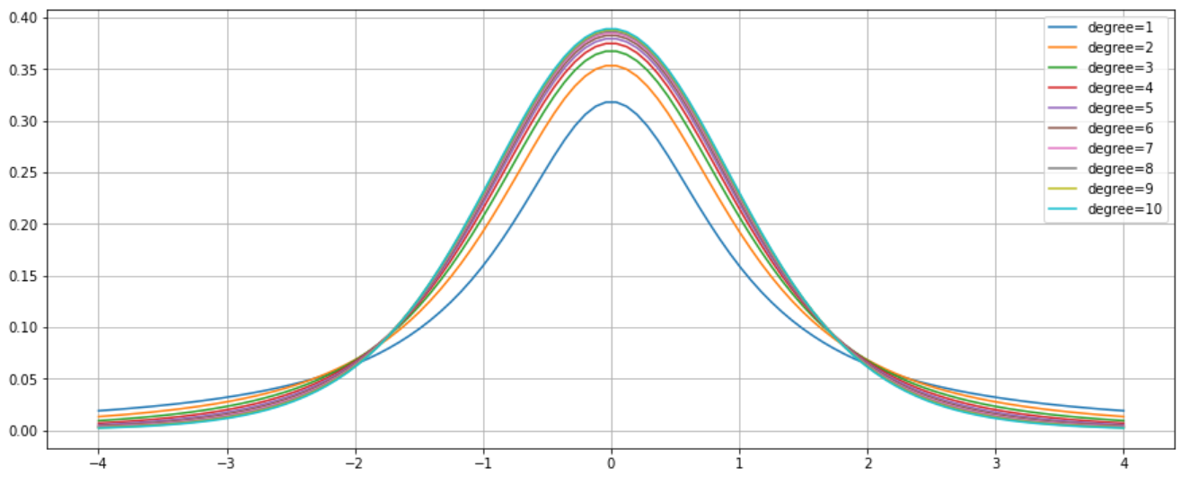
We got as a refresher that we will read the t-value, or the area above 3 with 35 degrees of freedom (
The probability density function for t distribution is:
where
Let’s calculate the area under t distribution to the right of 3.
percentile, _ = quad(t.pdf, 3.0, np.Inf, args=(35))This area turns out to be 0.2474%, and this probability is lower than alpha 5%. So our decision will still be the same, what we have observed under null hypothesis is highly unlikely to happen, this means that our assumption that the null hypothesis is correct is most likely to be false, so the null hypothesis should be rejected.
Conclusion
Hypothesis testing is important not just in data science, but in every field. In this post, we know how to calculate the p-value by hand and also by using Python. Happy learning! Cheers!