Viterbi Algorithm for HMM Decoding

Introduction

Viterbi Algorithm is usually used to find the most likely sequence in HMM. It is now also commonly used in speech recognition, speech synthesis, diarization, keyword spotting, computational linguistics, and bioinformatics. This semester, in the course “Speech Technology”, the acoustic signal is treated as the observed sequence of events, and a string of text is considered to be the hidden cause of the acoustic signal in speech recognition task. The Viterbi algorithm finds the most likely string of text given the acoustic signal.

Part-of-Speech

Viterbi algorithm allows us to solve HMM more efficiently than brute force approach. In this post, I am going to take part-of-speech tagging task as an example for Viterbi algorithm.

In NLP, part-of-speech tagging is basically saying that, for every word we see, commonly listed English parts of speech are noun, verb, adjective, adverb, pronoun, preposition, conjunction, interjection, numeral, article, or determiner. In this article, I want to make it simple, so I will just limit the options for each word, however, in general we will have lots of options for each word potentially, and we might have many words to deal with.

The standard HMM relies on 3 main assumptions:

1. Markovianity: The current state of the unobserved node depends solely upon the previous state of the unobserved variable.
2. Output Independence: The current state of the observed node depends solely upon the current state of the unobserved variable.
3. Stationarity: The transition probabilities are independent of time.

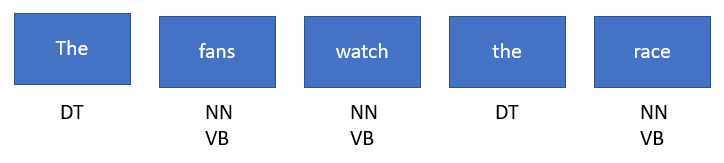
Let’s see this simple sentence below.

The Hidden Markov Model says that we have some hidden part-of-speech through , and these hidden part-of-speech have transition from one to the next, and generate these observed states (THE FANS WATCH THE RACE). So these vertical arrows are emission probabilities and horizontal arrows are transition probabilities.

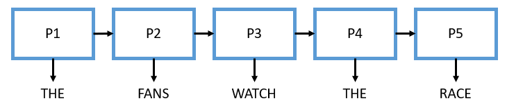
We could solve this problem if we were able to maximise the joint probability below.

The joint probability tells us what is the probability of observing both the observe states (THE FANS WATCH THE RACE) and also some setting of the hidden states (), and iterating over all possible combinations of the hidden states through .

It’s actually a bit harder to work in this form, becuase its’ a little bit unclear how to calculate this probability, but we can start incorporating the structure of the HMM, and write this in another form.

In this form, there are two distinct terms, the first one being the transition probabilities from one hidden state to the next, and the second term being the emission probabilities answering the question of “given the part-of-speech, what is the probability of seeing the corresponding word.”

Transition and Emission

Now, we are going to put some actual numbers for these transition and emission probabilities, so we can start solving this problem.

Transition Matrix

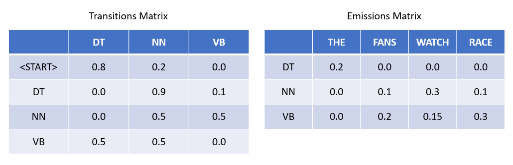
How to read the rows of transitions matrix? The rows are the last hidden state or the last part-of-speech for the previous word, and the columns are the part-of-speech for the current word. For example, 0.9 in the matrix means that if the current word is a determiner like “THE”, then there’s a 90% chance the next word will be a noun. We can make this is a valid transition matrix by making sure the rows add up to 1. Because given any state, we need to have a total of 100% probability of going to any of the other states. Another thing to claim is that I didn’t include all the possible part-of-speech tags in English language, but this is our transition matrix for now.

Emission Matrix

The other part is getting those emission probabilities, and those are enumerated in the right matrix. Similarly, the rows are the part-of-speech and the columns are the words. Take 0.15 for example, it says that, if you know the word is a verb, there’s a 15% chance that the generated observed word is “WATCH.” Another question you might have is that, how come the rows of this emission matrix don’t add up to 1. It’s becuase these empirical matrices (transition matrix and emission matrix) come from data, so we have some sort of underlying training set where we have the part-of-speech label made by linguistic expert, and we’re using that to generate these transition and emission probabilities. In that training data we obviously have more words than just these five words I take for instance in this article. So if we were to enumerate all of those words, even the ones that don’t occur in this specific example, then the rows in emission matrix will add up to 1.

There’s another interesting thing to note is that, if we use a more simple version of part-of-speech tagging where we didn’t take HMM property or the direction of the sentence into account, let’s say we did it based on emission probabilities alone. To highlight that, for the word “THE” it’s more likely to be a determiner, for the word “FANS” it’s more likely to be a verb, for the word “WATCH” it’s more likely to be a noun, for the word “RACE” it’s more likely to be a verb. If we choose “FANS” as a verb, “WATCH” as a noun, “RACE” as a verb in this context, all of them will be wrong. As a result, we know that it’s important to take the structure of the sentence into account. You’ll see that when working out the Viterbi algorithm. We’ll see very different result than looking at just the emission probabilities.

Viterbi Algorithm

Let’s put a diagram to help us walk through the exact mechanics of the Viterbi algorithm for this specific sentence.

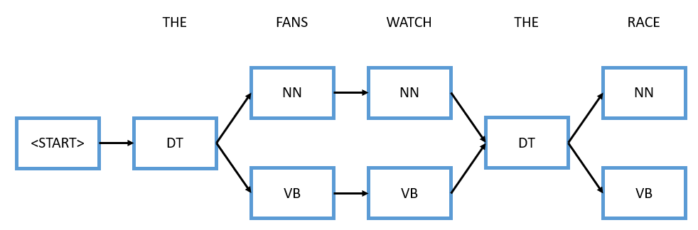
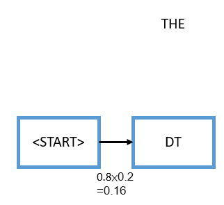
We start at the beginning, we have this starting tag , and we’re going to ask the first question which is given that we just started the sentence, what’s the probability that the first word is a determiner and given it’s a determiner that it’s the word “THE.” The first question comes from transition probabilities and the second question comes from emission probabilities. So we’re going to search for two numbers from these two matrices, and multiply them together. The first question is answered by given we just started the sentence, there’s a 80% chance that the first word is a determiner. For the second question, given that it’s a determiner, there’s a 20% of chance it’s the word “THE.”

Now we arrive at the word “FANS”, and “FANS” as we said before can either be a noun or a verb, so we need to consider both options. We will walk through the two options in the exact same way. First, pretend that we assigned “FANS” as a noun. Now the decision comes with two probabilities, first what’s the probability that we go from a determiner to a noun which is 0.9 from the transition probabilities, and second, given it’s a noun what’s the probability that generated the word “FANS” which would be 0.1 from the emission probabilities. We multiply these two terms with the existing 0.16, and we get 0.0144. Similarly, the other option is to consider “FANS” as a verb, we do the same process, so the first term will be 0.1 from the transition probabilities and the second term will be 0.2 from the emission probabilities. We multiply these two terms with the existing 0.16, and we get 0.0032.

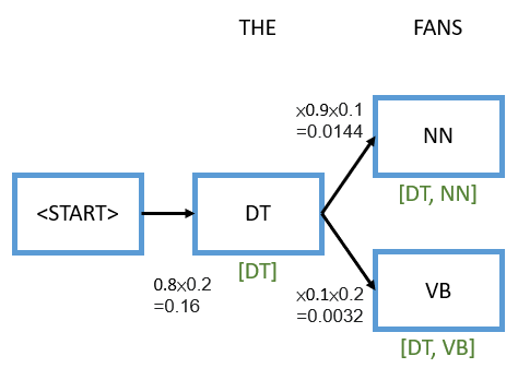
You might have a confusion point here. How come we can’t just stop the branch that has a lower probability, so we don’t have to consider anything after that. For instance, 0.0144 is clearly higher than 0.0032, so the question is how come we can’t just discontinue this branch and just go through the upper branch? The reason we can’t do that right now is that we don’t know what’s going to come next. It’s possible that even through this higher probabliity right now, based on the next step in this chain, that prbability might go to somewhere lower, so we can’t cut off this branch just yet, instead, we need to keep both these options in mind.

The next junction becomes more complex. Let’s dig into it. For the word “WATCH”, it can either be a noun or a verb. Furthermore, we can arrive at those two from different places, so you can see four total arrows in this junction here. The mechanics here is the same, so if you follow any one arrow, you’re going to have two terms again (transition and emission). For example, let’s consider noun goes to noun. We would multiply the transition probability of a noun going to a noun which is 0.5 by the emission probability which is given it’s a noun it generates the word “WATCH” which is 0.3. If we multiply these together on top of the point 0.0144, we get 0.00216. That’s not the only way to arrive at this noun node, we can also arrive at it from verb to noun. In that case, we do a very similar thing, we multiply the transition probability of 0.5 by the emission probability of 0.3, and we get 0.00048.

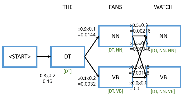
Let’s pause here and think for a second, notice there’s two ways to arrive at this word noun, one of those ways gave a total probability of 0.00216, the other gave a total probability of 0.00048. The one that’s higher is clearly the one on top that goes from determiner to noun to noun instead of going from determiner to verb to noun. At this point, we can confidently discontinue the path that had the lower probability. Why? Because from here no matter where the sentence procees from this node, we always get a higher probability if we only consider the path that has the maximum probability so far.

We do the same analysis for the downward path, and we get 0.00108 which is from determiner to noun to verb and 0.0 which is from determiner to verb to verb. And by the way, the part-of-speech that relates to this one would be [DT, NN, VB].

The rest of this will be more easy for you to continue, and I’ll just simply illustrate it in the diagram.

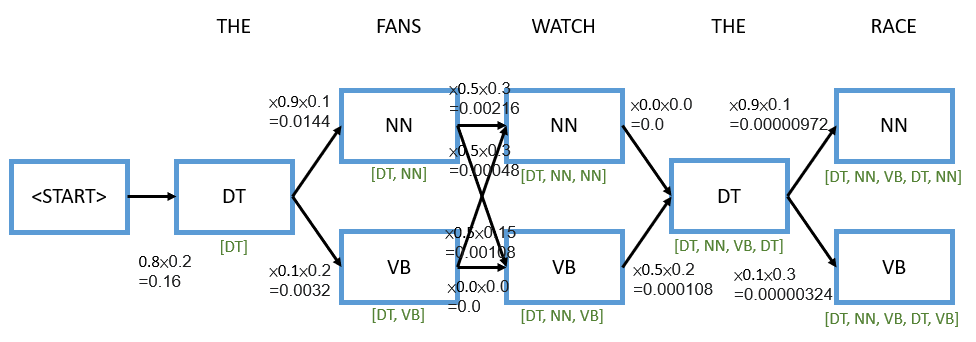
In the end, we have [DT, NN, VB, DT, NN], so we have successfully done part-of-speech tagging of this pretty simple sentence using the Viterbi algorithm.

Conclusion

Why is the Viterbi algorithm better than brute force approach? Assume we have P part-of-speech options and sentence of length L. So we have P nodes at each steps that we can consider like noun, verbs, etc, and the total length of our sequence is going to be L wide. If we did a brute force search, the big O complexity of this will be , because we have P options at each step and we have L steps, so if we’re going to consider all the possible paths, then we’ll get . Clearly, exponential growth is not smart way for any problem, we’re going to have efficiency issues. Now the Viterbi algorithm comes to the rescue. For one specific node, we know that we’re only going to consider the maximum probability path to get into that node, and all other options are discontinued from that node. Whereas the brute force approach would not discontinue then, instead, it would just search for all the exponentially growing paths. So for each layer, we have P possible way for each node, which ends up with ways for each layer. To be more specific, for each word, we have operations we need to do. There’s L words in total, so we have operations we have to do in general, which is clearly better than brute force approach.

References

1. https://www.cl.cam.ac.uk/teaching/1617/MLRD/slides/slides9.pdf
2. https://www.youtube.com/watch?v=IqXdjdOgXPM&ab_channel=ritvikmath
3. https://zhuanlan.zhihu.com/p/159363722
4. https://warwick.ac.uk/fac/sci/masdoc/current/msc-modules/ma916/mlia/hmm