Sentiment Analysis for Japanese Customer Reviews

Introduction

The development of elec-tronic business is accelerated by the popularity of the internet. Millions of people buy products and post their reviews online. Public opinion analysis can be used with these reviews. Customers can make better decisions after reading other people’s product reviews. There is a pressing need for building the system which can perform the sentiment classification job. In this article, I’ll try to build a sentiment anaylsis model for Japanese customer reviews.

Data

The dataset can be download from Darkmap’s GitHub here. The dataset used in this project consists of 20K reviews of commodities in various categories from Amazon Japan. The annotating is based on the rating of the reviews, since the scale of the corpus is too large for manual annotation. Reviews with rating 1 and 2 are considered negative while those with rating 4 and 5 are annotated as positive ones.

Import the Libraries

We will use SpaCy as our tokeniser, and use PyTorch to build the model.

import requests
import spacy
import numpy as np
import pandas as pd
import matplotlib.pyplot as plt
import seaborn as sns
from tqdm import tqdm
from collections import Counter
from sklearn import metrics
ja = spacy.blank('ja')

---

import torch
import torch.nn as nn
import torch.nn.functional as F
import torch.optim as optim
from torch.utils.data import Dataset, DataLoader

Load the Data

Utilise requests library to get the data.

positive_url = "https://raw.githubusercontent.com/Darkmap/japanese_sentiment/master/data/10000positive.txt"
negative_url = "https://raw.githubusercontent.com/Darkmap/japanese_sentiment/master/data/10000negative.txt"
positive_res = requests.get(positive_url)
negative_res = requests.get(negative_url)
positive_data = positive_res.text
negative_data = negative_res.text

The size for both positive and negative reviews are 10000.

positive_list = positive_data.split("\n")
positive_list = positive_list[:10000]

negative_list = negative_data.split("\n")
negative_list = negative_list[:10000]

Text Pre-processing

Before text was used as an input through the model, it’s necessary to convert the tokenised input data into an appropriate format so that each sentence can be sent to the model to obtain the corresponding embedding. This article introduces how text pre-processing can be done step by step.

Tokenisation

SpaCy’s trained pipelines can be installed as Python packages. SpaCy also provides support for vast languages including Japanese. You can take a look at the documentation for different language models.

There’s also another option to tokenise the Japanese sentence. MeCab is a Japanese word segmentation system developed by Taku Kudo of Nara Institute of Science and Technology. The basic approach of the design is to use Conditional Random Fields (CRF) models for parameter estimation without relying on specific languages, dictionaries, and corpora. Furthermore. Furthermore, the average parsing speed is higher than those of ChaSen, Juman, KAKASI and other Japanese lexical parsers. By the way, MeCab (めかぶ) is the author’s favorite food.

The first hurdle in analysing Japanese text is tokenisation. You can separate all the word boundaries of the European languages and English. Japanese, however, has no spaces in its text, so there’s an extra pre-processing step required before we can start using these text analysis approaches. In essence, we want to turn a string like this:

“今日はいい天気ですね。遊びに行かない？新宿で祭りがある！”

into an list like this:

[“今日”,　“は”,　“いい”,　“天気”,　“です”,　“ね”,　“遊び”,　“に”,　“行か”,　“ない”,　“新宿”,　“で”,　“祭り”,　“が”,　“ある”]

The next step is to get SpaCy talking to Python. Try the following code:

positive_tokenised, positive_part_of_speech = [], []
for doc in positive_list:
    temp_word, temp_pos = [], []
    for word in ja(doc.replace(" ", "")):
        temp_word.append(str(word))
        temp_pos.append(word.pos_)
    positive_tokenised.append(temp_word)
    positive_part_of_speech.append(temp_pos)
    
negative_tokenised, negative_part_of_speech = [], []
for doc in negative_list:
    temp_word, temp_pos = [], []
    for word in ja(doc.replace(" ", "")):
        temp_word.append(str(word))
        temp_pos.append(word.pos_)
    negative_tokenised.append(temp_word)
    negative_part_of_speech.append(temp_pos)

Here in my experiment, I am trying to add more features in the model, so you can see that I also extract the part-of-speech tagging in the above code chunk. Later when building the model, I will employ some different features including part-of-speech tag (POS tag). The POS tag feature share the same characteristics as the word embedding feature. It has time series information and needs to be processed over time per-token.

Extract N-Grams

After tokenise all the sentences in the documents, next step is to extract all n-grams. First, I’ll implement the extract_ngrams() function. It takes as input:

• x_raw: a string corresponding to the raw text of a document.
• ngram_range: a tuple of two integers denoting the type of n-grams you want to extract, e.g. (1, 2) denotes extracting unigrams and bigrams.
• stop_words: a list of stop words.
• vocab: a given vocabulary. It should be used to extract specific features.

and returns a list of all extracted features.

def extract_ngrams(x_raw, 
                   ngram_range=(1, 3), 
                   stop_words=[], 
                   vocab=set()):
    
    # First extract all unigrams by tokenising
    x_uni = [w for w in x_raw.split() if w not in stop_words]
    
    # This is to store the ngrams to be returned
    x = []
    
    if ngram_range[0]==1:
        x = x_uni

    # Generate n-grams from the available unigrams x_uni
    ngrams = []
    for n in range(ngram_range[0], ngram_range[1]+1):

    # Ignore unigrams
        if n==1: continue

        # Pass a list of lists as an argument for zip
        arg_list = [x_uni]+[x_uni[i:] for i in range(1, n)]

        # Extract tuples of n-grams using zip
        x_ngram = list(zip(*arg_list))
        ngrams.append(x_ngram)

    for n in ngrams:
        for t in n:
            x.append(t)

    if len(vocab)>0:
        x = [w for w in x if w in vocab]
        
    return x

Create Vocabulary of N-Grams and POS Tag

Then the get_vocab() function will be used to (1) create a vocabulary of ngrams; (2) count the document frequencies of ngrams; (3) their raw frequency. It takes as input:

• X_raw: a list of strings each corresponding to the raw text of a document.
• ngram_range: a tuple of two integers denoting the type of n-grams you want to extract, e.g. (1, 2) denotes extracting unigrams and bigrams.
• min_df: keep n-grams with a minimum document frequency.
• keep_topN: keep top-N more frequent n-grams.
• stop_words: a list of stop words.

and returns:

• vocab: a set of the n-grams that will be used as features.
• df: a Counter (or dict) that contains n-grams as keys and their corresponding document frequency as values.
• ngram_counts: counts of each n-gram in vocab.

def get_vocab(X_raw, 
              ngram_range=(1, 3), 
              min_df=0, 
              keep_topN=0, 
              stop_words=[]):
    
    df = Counter()
    ngram_counts = Counter()
    vocab = set()
    
    # Iterate through each raw text
    for x in X_raw:
        
        x_ngram = extract_ngrams(x, 
                                 ngram_range=ngram_range, 
                                 stop_words=stop_words)
        
        # Update doc and ngram frequencies 
        df.update(list(set(x_ngram)))
        ngram_counts.update(x_ngram)

    # Obtain a vocabulary as a set. 
    # Keep elements with doc frequency > minimum doc freq (min_df)
    # Note that df contains all te
    vocab = set([w for w in df if df[w]>=min_df])
    
    # Keep the top N most freqent 
    if keep_topN > 0:
        vocab = set([w[0] for w in ngram_counts.most_common(keep_topN) 
                     if w[0] in vocab])
    
    return vocab, df, ngram_counts

Now we could use get_vocab() to create the vocabulary and get document and raw frequencies of n-grams:

# Create vocab for documents
positive_doc = [" ".join(doc) for doc in positive_tokenised]
negative_doc = [" ".join(doc) for doc in negative_tokenised]
vocab, df, ngram_counts = get_vocab(positive_doc+negative_doc, 
                                    ngram_range=(1, 1), 
                                    min_df=0, 
                                    keep_topN=0, 
                                    stop_words=[])

# Create vocab for pos tag
positive_doc_pos = [" ".join(doc) for doc in positive_part_of_speech]
negative_doc_pos = [" ".join(doc) for doc in negative_part_of_speech]
pos_vocab, _, _ = get_vocab(positive_doc_pos+negative_doc_pos, 
                            ngram_range=(1, 1), 
                            min_df=0, 
                            keep_topN=0, 
                            stop_words=[])

The sizes of the vocabulary are 18347 and 17 of documents and pos tagging, respectively.

Then, you need to create vocabulary idx2word, word2idx, idx2pos, and pos2idx dictionaries for reference:

idx2word = {k+4:v for k, v in enumerate(vocab)}
idx2word[0] = "<PAD>"
idx2word[1] = "<CLS>"
idx2word[2] = "<EOS>"
idx2word[3] = "<UNK>"
word2idx = {v:k for k, v in idx2word.items()}

idx2pos = {k:v for k, v in enumerate(pos_vocab)}
pos2idx = {v:k for k, v in idx2pos.items()}

where the first four tokens in idx2word represent:

• <PAD>: your GPU (or CPU at worst) processes your training data in batches and all the sequences in your batch should have the same length. If the max length of your sequence is 8, your sentence You had me at hello will be padded from either side to fit this length: You had me at hello
• <CLS>: CLS stands for “classification” and its there to represent sentence-level classification.
• <EOS>: EOS stands for “end of sentence”.
• <UNK>: UNK stands for “unknown token”, and is used to replace the rare words that did not fit in your vocabulary. So your sentence She suffered an extreme case of Kakorrhaphiophobia will be translated into She suffered an extreme case of .

Split the Dataset

The hold-out method is the simplest kind of cross validation. Hold-out is when you split up your dataset into several parts. In order to train and validate a model, you must first partition your dataset, which involves choosing what percentage of your data to use for the training, validation, and holdout sets.

What is a Training Set?

A training set is the subsection of a dataset from which the machine learning algorithm uncovers, or “learns”” relationships between the features and the target variable. In supervised machine learning, training data is labeled with known outcomes.

What is a Validation Set?

A validation set is another subset of the input data to which we apply the machine learning algorithm to see how accurately it identifies relationships between the known outcomes for the target variable and the dataset’s other features.

What is a Holdout Set?

Sometimes referred to as “testing” data, a holdout subset provides a final estimate of the machine learning model’s performance after it has been trained and validated. Holdout sets should never be used to make decisions about which algorithms to use or for improving or tuning algorithms.

Hold-out Validation vs. Cross-Validation

By the way, Andrew Ng mentioned in the CS229 class at University of Stanford regarding cross-validation. These are the practices that he follow in his own work. Let m be the number of samples in your dataset.

1. If , then use Leave-one-out cross-validation.
2. If , then use k-fold cross-validation with a relatively large
3. If , then use regular k-fold cross-validation (). Or, if there is not enough computational power and , then use hold-out cross-validation.
4. If , then use hold-out validation. But if computational power is available you can use k-fold cross-validation () if you want to squeeze that extra performance out of your model.

In this project, I have 20000 of samples in total, so I’ll just use basic hold-out validation. 16000 of samples for training dataset, 2000 for validation dataset, and 2000 for testing dataset.

train_documents = positive_doc[:8000] + negative_doc[:8000]
valid_documents = positive_doc[8000:9000] + negative_doc[8000:9000]
test_documents = positive_doc[9000:] + negative_doc[9000:]

train_pos = positive_doc_pos[:8000] + negative_doc_pos[:8000]
valid_pos = positive_doc_pos[8000:9000] + negative_doc_pos[8000:9000]
test_pos = positive_doc_pos[9000:] + negative_doc_pos[9000:]

train_label = [1]*8000 + [0]*8000
valid_label = [1]*1000 + [0]*1000
test_label = [1]*1000 + [0]*1000

Convert the List of Unigrams into a List of Vocab Indices

Storing actual one-hot vectors into memory for all words in the entire data set is prohibitive.Instead, we will store word indices in the vocabulary and look-up the weight matrix. This isequivalent of doing a dot product between an one-hot vector and the weight matrix.

First, represent documents in train, dev and test sets as lists of words in the vocabulary:

train_idx_list = [[word2idx.get(token) for token in extract_ngrams(
    doc, 
    ngram_range=(1, 1), 
    stop_words=[], 
    vocab=vocab)] for doc in train_documents]

valid_idx_list = [[word2idx.get(token) for token in extract_ngrams(
    doc, 
    ngram_range=(1, 1), 
    stop_words=[], 
    vocab=vocab)] for doc in valid_documents]

test_idx_list = [[word2idx.get(token) for token in extract_ngrams(
    doc, 
    ngram_range=(1, 1), 
    stop_words=[], 
    vocab=vocab)] for doc in test_documents]

Second, represent POS tag in train, dev, and test sets as lists of tags in the POS vocabulary.

train_pos_idx_list = [[pos2idx.get(pos) for pos in extract_ngrams(
    doc, 
    ngram_range=(1, 1), 
    stop_words=[], 
    vocab=pos_vocab)] for doc in train_pos]

valid_pos_idx_list = [[pos2idx.get(pos) for pos in extract_ngrams(
    doc, 
    ngram_range=(1, 1), 
    stop_words=[], 
    vocab=pos_vocab)] for doc in valid_pos]

test_pos_idx_list = [[pos2idx.get(pos) for pos in extract_ngrams(
    doc, 
    ngram_range=(1, 1), 
    stop_words=[], 
    vocab=pos_vocab)] for doc in test_pos]

Seqeunce Padding

Padding comes from the need to encode sequence data into contiguous batches: in order to make all sequences in a batch fit a given standard length, it is necessary to pad or truncate some sequences. The function pad_sequence() pads sequences to the same length.

def pad_sequence(sequences, max_len=None):
    if max_len is not None:
        max_ = max([len(seq) for seq in sequences])
    return [seq + [0]*(max_len-len(seq)) 
    	if len(seq) < max_len else seq[:max_len] 
    	for seq in sequences]

The function pad_sequence() truncates and pads Python lists to a common length of 128 in our case.

MAX_LENGTH = 128

train_idx_list_padded = pad_sequence(train_idx_list, MAX_LENGTH)
valid_idx_list_padded = pad_sequence(valid_idx_list, MAX_LENGTH)
test_idx_list_padded = pad_sequence(test_idx_list, MAX_LENGTH)

train_pos_idx_list_padded = pad_sequence(train_pos_idx_list, MAX_LENGTH)
valid_pos_idx_list_padded = pad_sequence(valid_pos_idx_list, MAX_LENGTH)
test_pos_idx_list_padded = pad_sequence(test_pos_idx_list, MAX_LENGTH)

Dataset and Dataloader

We have to keep in mind that in some cases, even the most state-of-the-art configuration won’t have enough memory space to process the data the way we used to do it. That is the reason why we need to find other ways to do that task efficiently.

Dataset

Now, let’s go through the details of how to set the Python class Dataset, which will characterize the key features of the dataset you want to generate.

class ReviewsDataset(Dataset):
    
    def __init__(self, sequences, labels):
        self.sequences = sequences
        self.labels = labels

    def __len__(self):
        return len(self.labels)

    def __getitem__(self, index):
        seq = torch.LongTensor(self.sequences[index])
        label = torch.LongTensor([self.labels[index]])
        return seq, label
    
    def get_dataloader(self, batch_size, shuffle, num_workers=0):
        return DataLoader(self, batch_size=batch_size, shuffle=shuffle, num_workers=num_workers)

Each call requests a sample index for which the upperbound is specified in the __len__ method. When the sample corresponding to a given index is called, the generator executes the __getitem__ method to generate it.

BATCH_SIZE = 32
EPOCHS = 100

train_dataset = ReviewsDataset(train_idx_list_padded, train_label)
valid_dataset = ReviewsDataset(valid_idx_list_padded, valid_label)
test_dataset = ReviewsDataset(test_idx_list_padded, test_label)

Dataloader

Now, we have to modify our PyTorch script accordingly so that it accepts the generator that we just created. In order to do so, we use PyTorch’s DataLoader class, which in addition to our Dataset class, also takes in the following important arguments:

• batch_size: denotes the number of samples contained in each generated batch.
• shuffle: if set to True, we will get a new order of exploration at each pass (or just keep a linear exploration scheme otherwise).
• num_workers: denotes the number of processes that generate batches in parallel.

train_generator = train_dataset.get_dataloader(
	batch_size=BATCH_SIZE, shuffle=True)
valid_generator = valid_dataset.get_dataloader(
	batch_size=BATCH_SIZE, shuffle=False)
test_generator = test_dataset.get_dataloader(
	batch_size=BATCH_SIZE, shuffle=False)

Modeling

For specifying more complex neural network structure, we have to define our own modules by subclassing nn.Module and defining a forward which receives input tensors and produces output tensors using other modules or other autograd operations on tensors.

This implementation defines the model as a custom Module subclass. I’ll use EmbeddingBag as the baseline. The PyTorch EmbeddingBag operator computes sums or means of “bags” of embeddings. EmbeddingBag is the integration of look-up tables into an embedding. This is quite similar to FastText proposed by FaceBook.

There are three extra functions I created in this TextClassifier class.

1. fit: in a nutshell, fitting is equal to training. Then, after it is trained, the model can be used to make predictions.
2. predict: classify incoming data points.
3. plot: diagnose the behavior of a machine learning model. There are three common dynamics that you are likely to observe in learning curves; they are: underfit, overfit, and good fit.

class TextClassifier(nn.Module):
    
    #define all the layers used in model
    def __init__(self, 
                 vocab_size, 
                 embedding_dim, 
                 output_dim, 
                 dropout):
        
        super().__init__()
        self.embedding = nn.EmbeddingBag(vocab_size, embedding_dim)
        self.drop = nn.Dropout(dropout)
        self.fc = nn.Linear(embedding_dim, output_dim)
        self.output = nn.Sigmoid()
        
        self.epochs = None
        self.train_loss = None
        self.valid_loss = None
        
    def forward(self, text):
        embedded = self.embedding(text)
        dense_outputs = self.fc(self.drop(embedded))
        outputs = self.output(dense_outputs)
        return outputs
    
    def count_parameters(self):
        count = sum(p.numel() for p in self.parameters() if p.requires_grad)
        print(f'The model has {count:,} trainable parameters.')
        
    def fit(self, train_generator, valid_generator, criterion, optimiser, device, epochs=10):
        train_loss, valid_loss = [], []

        # Loop over epochs
        for epoch in tqdm(range(epochs)):
            # Training
            model.train()
            epoch_loss = 0
            for local_seqs, local_labels in train_generator:
                optimiser.zero_grad()
                local_seqs, local_labels = local_seqs.to(device), local_labels.to(device)
                predictions = self(local_seqs)
                loss = criterion(predictions.type(torch.float64), local_labels.type(torch.float64))
                loss.backward()       
                optimiser.step()      
                epoch_loss += loss.item()
            train_loss.append(epoch_loss / len(train_generator))

            # Validation
            model.eval()
            epoch_loss = 0
            with torch.set_grad_enabled(False):
                for local_seqs, local_labels in valid_generator:
                    # Transfer to GPU
                    local_seqs, local_labels = local_seqs.to(device), local_labels.to(device)
                    predictions = self(local_seqs)
                    loss = criterion(predictions.type(torch.float64), local_labels.type(torch.float64))
                    epoch_loss += loss.item()
                valid_loss.append(epoch_loss / len(valid_generator))
        
        self.epochs = epochs
        self.train_loss = train_loss
        self.valid_loss = valid_loss
        
    def predict(self, test_generator, device, threshold=0.5):
        predictions_list = []
        with torch.set_grad_enabled(False):
            for local_seqs, local_labels in test_generator:
                # Transfer to GPU
                local_seqs, local_labels = local_seqs.to(device), local_labels.to(device)
                predictions = self(local_seqs)
                predictions_list.append(predictions)
                
        test_preds = (torch.cat(predictions_list).detach().cpu().numpy() >= threshold).astype(int)
        test_preds = test_preds.reshape(-1, 1)
        return test_preds
        
    def plot(self):
        plt.figure(figsize=(15, 6))
        plt.plot(range(1, self.epochs+1), self.train_loss, label="train")
        plt.plot(range(1, self.epochs+1), self.valid_loss, label="valid")
        plt.legend()
        plt.grid()
        plt.show()

Training Process

I would like to train the model in four different aspects.

1. Without regularisation
2. With dropout
3. With L2 regularisation
4. With dropout and L2 regularisation

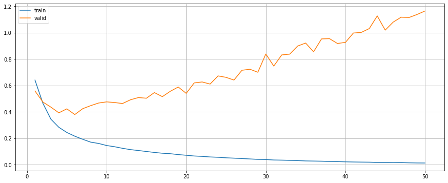
Train without Regularisation

model = TextClassifier(vocab_size=len(vocab), 
                       embedding_dim=300, 
                       output_dim=1, 
                       dropout=0.0)
optimiser = optim.Adam(model.parameters())
criterion = nn.BCELoss()

model.to(device)
criterion.to(device)

model.fit(train_generator, valid_generator, criterion, optimiser, device, epochs=50)
model.plot()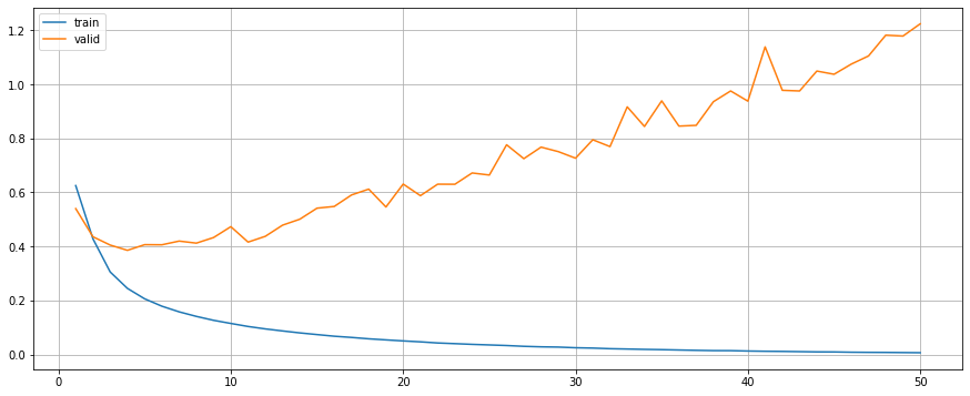

test_preds = model.predict(test_generator, device)
print(metrics.classification_report(test_label, test_preds))

print(f'Accuracy: {metrics.accuracy_score(test_label, test_preds): .4f}')
print(f'Precision: {metrics.precision_score(test_label, test_preds): .4f}')
print(f'Recall: {metrics.recall_score(test_label, test_preds): .4f}')
print(f'F1-Score: {metrics.f1_score(test_label, test_preds): .4f}')

---

              precision    recall  f1-score   support

           0       0.90      0.96      0.93      1000
           1       0.95      0.90      0.92      1000

    accuracy                           0.93      2000
   macro avg       0.93      0.93      0.93      2000
weighted avg       0.93      0.93      0.93      2000

Accuracy:  0.9270
Precision:  0.9533
Recall:  0.8980
F1-Score:  0.9248

Train with Regularisation (Dropout)

model = TextClassifier(vocab_size=len(vocab), 
                       embedding_dim=300, 
                       output_dim=1, 
                       dropout=0.25)
optimiser = optim.Adam(model.parameters())
criterion = nn.BCELoss()

model.to(device)
criterion.to(device)

model.fit(train_generator, valid_generator, criterion, optimiser, device, epochs=50)
model.plot()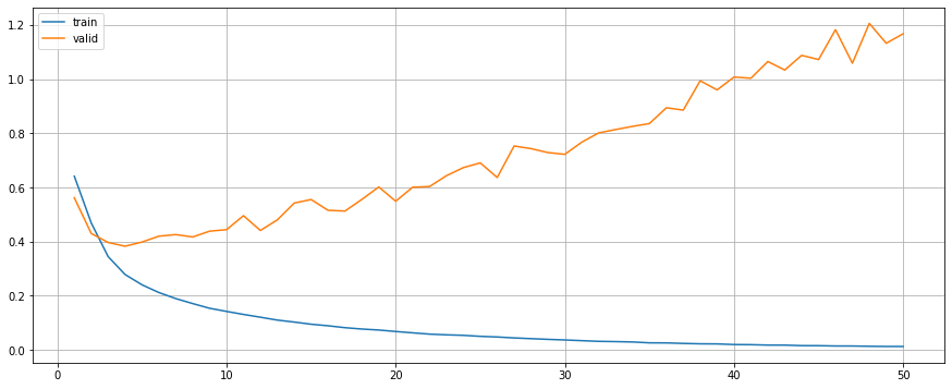

test_preds = model.predict(test_generator, device)
print(metrics.classification_report(test_label, test_preds))

print(f'Accuracy: {metrics.accuracy_score(test_label, test_preds): .4f}')
print(f'Precision: {metrics.precision_score(test_label, test_preds): .4f}')
print(f'Recall: {metrics.recall_score(test_label, test_preds): .4f}')
print(f'F1-Score: {metrics.f1_score(test_label, test_preds): .4f}')

---

              precision    recall  f1-score   support

           0       0.91      0.96      0.93      1000
           1       0.96      0.91      0.93      1000

    accuracy                           0.93      2000
   macro avg       0.93      0.93      0.93      2000
weighted avg       0.93      0.93      0.93      2000

Accuracy:  0.9320
Precision:  0.9567
Recall:  0.9050
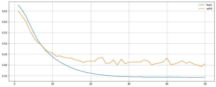
F1-Score:  0.9301

Train with Regularisation (L2)

model = TextClassifier(vocab_size=len(vocab), 
                       embedding_dim=300, 
                       output_dim=1, 
                       dropout=0.0)
optimiser = optim.Adam(model.parameters(), weight_decay=1e-4)
criterion = nn.BCELoss()

model.to(device)
criterion.to(device)

model.fit(train_generator, valid_generator, criterion, optimiser, device, epochs=50)
model.plot()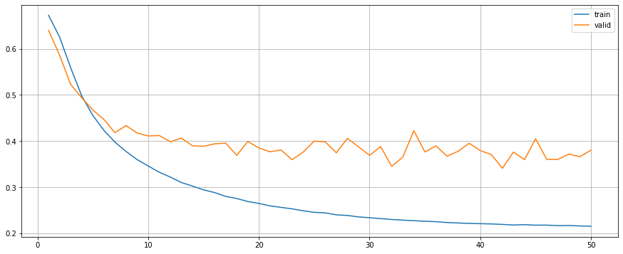

test_preds = model.predict(test_generator, device)
print(metrics.classification_report(test_label, test_preds))

print(f'Accuracy: {metrics.accuracy_score(test_label, test_preds): .4f}')
print(f'Precision: {metrics.precision_score(test_label, test_preds): .4f}')
print(f'Recall: {metrics.recall_score(test_label, test_preds): .4f}')
print(f'F1-Score: {metrics.f1_score(test_label, test_preds): .4f}')

---

              precision    recall  f1-score   support

           0       0.88      0.96      0.92      1000
           1       0.96      0.87      0.91      1000

    accuracy                           0.92      2000
   macro avg       0.92      0.92      0.92      2000
weighted avg       0.92      0.92      0.92      2000

Accuracy:  0.9160
Precision:  0.9561
Recall:  0.8720
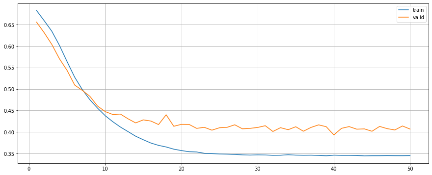
F1-Score:  0.9121

Train with Regularisation (Dropout + L2)

model = TextClassifier(vocab_size=len(vocab), 
                       embedding_dim=300, 
                       output_dim=1, 
                       dropout=0.25)
optimiser = optim.Adam(model.parameters(), weight_decay=1e-4)
criterion = nn.BCELoss()

model.to(device)
criterion.to(device)

model.fit(train_generator, valid_generator, criterion, optimiser, device, epochs=50)
model.plot()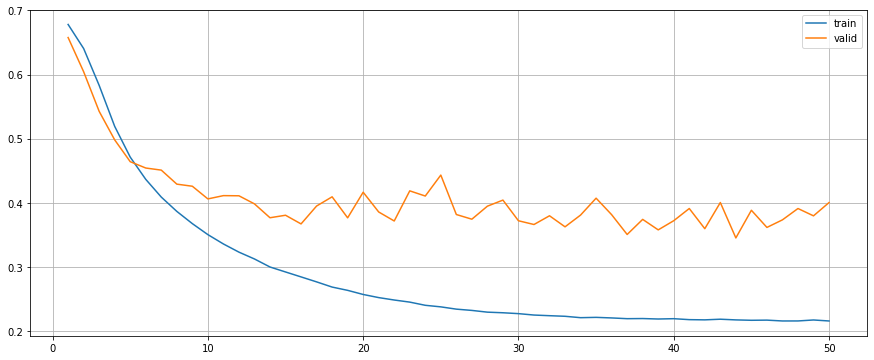

test_preds = model.predict(test_generator, device)
print(metrics.classification_report(test_label, test_preds))

print(f'Accuracy: {metrics.accuracy_score(test_label, test_preds): .4f}')
print(f'Precision: {metrics.precision_score(test_label, test_preds): .4f}')
print(f'Recall: {metrics.recall_score(test_label, test_preds): .4f}')
print(f'F1-Score: {metrics.f1_score(test_label, test_preds): .4f}')

---

              precision    recall  f1-score   support

           0       0.91      0.94      0.93      1000
           1       0.94      0.91      0.92      1000

    accuracy                           0.93      2000
   macro avg       0.93      0.93      0.93      2000
weighted avg       0.93      0.93      0.93      2000

Accuracy:  0.9260
Precision:  0.9401
Recall:  0.9100
F1-Score:  0.9248

Performance

Although model with dropout outperms others, it seems to be overfitting. While the model with L2 and the model with both dropout and L2 have a better learning curve during the training process.

Model	Accuracy	Precision	Recall	F1-Score
Without Reg	0.9270	0.9533	0.8980	0.9248
With Dropout	0.9320	0.9567	0.9050	0.9301
With L2	0.9160	0.9561	0.8720	0.9121
With Dropout & L2	0.9260	0.9401	0.9100	0.9248

Word Embedding and POS Embedding

Add the POS tags as a features to the embedding vectors. I guess extending word vectors with POS tags is a good practice, because it could deal with polysemy, for example. In Lasguido Nio and Koji Murakami’s paper “Japanese Sentiment Classification Using Bidirectional Long Short-Term Memory Recurrent Neural Network”, they appended the network hidden layer with the Part
of Speech tag (POStag) feature and Japanese polarity dictionary information. Their model achieves the state-of-the-art performance in Japanese sentiment classification task. Therefore, I want to give a try implementing their idea on different dataset.

Basically, there’s not much difference in building Dataset and Dataloader subclass.

class ReviewsPOSDataset(Dataset):
    
    def __init__(self, sequences, tags, labels):
        self.sequences = sequences
        self.tags = tags
        self.labels = labels

    def __len__(self):
        return len(self.labels)

    def __getitem__(self, index):
        seq = torch.LongTensor(self.sequences[index])
        tag = torch.LongTensor(self.tags[index])
        label = torch.LongTensor([self.labels[index]])
        return seq, tag, label
    
    def get_dataloader(self, batch_size, shuffle, num_workers=0):
        return DataLoader(self, batch_size=batch_size, shuffle=shuffle, num_workers=num_workers)

---

train_pos_dataset = ReviewsPOSDataset(
	train_idx_list_padded, train_pos_idx_list_padded, train_label)
valid_pos_dataset = ReviewsPOSDataset(
	valid_idx_list_padded, valid_pos_idx_list_padded, valid_label)
test_pos_dataset = ReviewsPOSDataset(
	test_idx_list_padded, test_pos_idx_list_padded, test_label)

train_pos_generator = train_pos_dataset.get_dataloader(
	batch_size=BATCH_SIZE, shuffle=True)
valid_pos_generator = valid_pos_dataset.get_dataloader(
	batch_size=BATCH_SIZE, shuffle=False)
test_pos_generator = test_pos_dataset.get_dataloader(
	batch_size=BATCH_SIZE, shuffle=False)

Next, build the model.

class TextPOSClassifier(nn.Module):
    
    #define all the layers used in model
    def __init__(self, 
                 vocab_size, 
                 embedding_dim, 
                 pos_size, 
                 pos_embedding_dim, 
                 output_dim, 
                 dropout):
        
        super().__init__()
        self.device = device
        self.embedding = nn.EmbeddingBag(vocab_size, embedding_dim)
        self.pos_embedding = nn.EmbeddingBag(pos_size, pos_embedding_dim)
        self.linear1 = nn.Linear(embedding_dim, int((embedding_dim+pos_embedding_dim)/2))
        self.linear2 = nn.Linear(pos_embedding_dim, int((embedding_dim+pos_embedding_dim)/2))
        self.drop = nn.Dropout(dropout)
        self.fc = nn.Linear(int((embedding_dim+pos_embedding_dim)/2), output_dim)
        self.output = nn.Sigmoid()
        
    def forward(self, text, tag):
        text_embedded = self.embedding(text)
        pos_embedded = self.pos_embedding(tag)
        text_embedded = self.linear1(text_embedded)
        pos_embedded = self.linear2(pos_embedded)
        embedded = torch.add(text_embedded, pos_embedded)
        dense_outputs = self.fc(self.drop(embedded))
        outputs = self.output(dense_outputs)
        return outputs
    
    def count_parameters(self):
        count = sum(p.numel() for p in self.parameters() if p.requires_grad)
        print(f'The model has {count:,} trainable parameters.')
        
    def fit(self, train_generator, valid_generator, criterion, optimiser, device, epochs=10):
        train_loss, valid_loss = [], []

        # Loop over epochs
        for epoch in tqdm(range(epochs)):
            # Training
            model.train()
            epoch_loss = 0
            for local_seqs, local_tags, local_labels in train_generator:
                optimiser.zero_grad()
                local_seqs, local_labels = local_seqs.to(device), local_labels.to(device)
                local_tags = local_tags.to(device)
                predictions = self(local_seqs, local_tags)
                loss = criterion(predictions.type(torch.float64), local_labels.type(torch.float64))
                loss.backward()       
                optimiser.step()      
                epoch_loss += loss.item()
            train_loss.append(epoch_loss / len(train_generator))

            # Validation
            model.eval()
            epoch_loss = 0
            with torch.set_grad_enabled(False):
                for local_seqs, local_tags, local_labels in valid_generator:
                    # Transfer to GPU
                    local_seqs, local_labels = local_seqs.to(device), local_labels.to(device)
                    local_tags = local_tags.to(device)
                    predictions = self(local_seqs, local_tags)
                    loss = criterion(predictions.type(torch.float64), local_labels.type(torch.float64))
                    epoch_loss += loss.item()
                valid_loss.append(epoch_loss / len(valid_generator))
        
        self.epochs = epochs
        self.train_loss = train_loss
        self.valid_loss = valid_loss
        
    def predict(self, test_generator, device, threshold=0.5):
        predictions_list = []
        with torch.set_grad_enabled(False):
            for local_seqs, local_tags, local_labels in test_generator:
                # Transfer to GPU
                local_seqs, local_labels = local_seqs.to(device), local_labels.to(device)
                local_tags = local_tags.to(device)
                predictions = self(local_seqs, local_tags)
                predictions_list.append(predictions)
                
        test_preds = (torch.cat(predictions_list).detach().cpu().numpy() >= threshold).astype(int)
        test_preds = test_preds.reshape(-1, 1)
        return test_preds
        
    def plot(self):
        plt.figure(figsize=(15, 6))
        plt.plot(range(1, self.epochs+1), self.train_loss, label="train")
        plt.plot(range(1, self.epochs+1), self.valid_loss, label="valid")
        plt.legend()
        plt.grid()
        plt.show()

I will only show the performance table over here, because the training code is exactly the same as the previous.

Model	Accuracy	Precision	Recall	F1-Score
Without Reg	0.9305	0.9415	0.9180	0.9296
With Dropout	0.9320	0.9435	0.9190	0.9311
With L2	0.9360	0.9658	0.9040	0.9339
With Dropout & L2	0.9365	0.9619	0.9090	0.9347

As you can see in the table, after adding POS embedding to the model, it can perform better.

Grid Search

The traditional way of performing hyperparameter optimization has been grid search, or a parameter sweep, which is simply an exhaustive searching through a manually specified subset of the hyperparameter space of a learning algorithm.

from itertools import product

PARAMS = {
    "batch_size": [16, 32], 
    "embedding_dim": [100, 300], 
    "pos_embedding_dim": [100, 300], 
    "dropout": [0.0, 0.25]
}

results = []
for batch_size, embedding_dim, pos_embedding_dim, dropout in product(*[v for v in PARAMS.values()]):
    train_pos_dataset = ReviewsPOSDataset(train_idx_list_padded, train_pos_idx_list_padded, train_label)
    valid_pos_dataset = ReviewsPOSDataset(valid_idx_list_padded, valid_pos_idx_list_padded, valid_label)
    test_pos_dataset = ReviewsPOSDataset(test_idx_list_padded, test_pos_idx_list_padded, test_label)

    train_pos_generator = train_pos_dataset.get_dataloader(batch_size=batch_size, shuffle=True)
    valid_pos_generator = valid_pos_dataset.get_dataloader(batch_size=batch_size, shuffle=False)
    test_pos_generator = test_pos_dataset.get_dataloader(batch_size=batch_size, shuffle=False)
    
    model = TextPOSClassifier(vocab_size=len(vocab), 
                              embedding_dim=embedding_dim, 
                              pos_size=len(pos_vocab), 
                              pos_embedding_dim=pos_embedding_dim, 
                              output_dim=1, 
                              dropout=dropout)
    optimiser = optim.Adam(model.parameters(), weight_decay=3e-4)
    criterion = nn.BCELoss()
    model.to(device)
    criterion.to(device)
    model.fit(train_pos_generator, valid_pos_generator, criterion, optimiser, device, epochs=40)
    
    test_preds = model.predict(test_pos_generator, device)
    accuracy = metrics.accuracy_score(test_label, test_preds)
    precision = metrics.precision_score(test_label, test_preds)
    recall = metrics.recall_score(test_label, test_preds)
    f1 = metrics.f1_score(test_label, test_preds)
    results.append([batch_size, embedding_dim, pos_embedding_dim, accuracy, precision, recall, f1])

index	batch_size	embedding_dim	pos_embedding_dim	accuracy	precision	recall	f1
0	16	100	100	0.9310	0.926733	0.936	0.931343
1	16	100	100	0.9395	0.965079	0.912	0.937789
2	16	100	300	0.9380	0.959119	0.915	0.936540
3	16	100	300	0.9300	0.968410	0.889	0.927007
4	16	300	100	0.9370	0.944106	0.929	0.936492
5	16	300	100	0.9360	0.957023	0.913	0.934493
6	16	300	300	0.9310	0.969499	0.890	0.928050
7	16	300	300	0.9320	0.929423	0.935	0.932203
8	32	100	100	0.9350	0.953125	0.915	0.933673
9	32	100	100	0.9335	0.962647	0.902	0.931337
10	32	100	300	0.9360	0.963830	0.906	0.934021
11	32	100	300	0.9325	0.940877	0.923	0.931853
12	32	300	100	0.9295	0.928215	0.931	0.929606
13	32	300	100	0.9275	0.918707	0.938	0.928253
14	32	300	300	0.9320	0.943532	0.919	0.931104
15	32	300	300	0.9125	0.888053	0.944	0.915172

Concatenate with Word Embedding and POS Embedding

In the last section, I built the model with adding up word embedding vectors and POS embedding vector. I was wondering if concatenating these two vectors would work as well.

Basically, we need to change two part of the code only.

class TextPOSConcatClassifier(nn.Module):
    
    #define all the layers used in model
    def __init__(self, 
                 vocab_size, 
                 embedding_dim, 
                 pos_size, 
                 pos_embedding_dim, 
                 output_dim, 
                 dropout):
        
        super().__init__()
        self.device = device
        self.embedding = nn.EmbeddingBag(vocab_size, embedding_dim)
        self.pos_embedding = nn.EmbeddingBag(pos_size, pos_embedding_dim)
        self.drop = nn.Dropout(dropout)
        self.fc = nn.Linear(embedding_dim+pos_embedding_dim, output_dim)
        self.output = nn.Sigmoid()
        
    def forward(self, text, tag):
        text_embedded = self.embedding(text)
        pos_embedded = self.pos_embedding(tag)
        embedded = torch.cat((text_embedded, pos_embedded), dim=1)
        dense_outputs = self.fc(self.drop(embedded))
        outputs = self.output(dense_outputs)
        return outputs

Train without Regularisation

              precision    recall  f1-score   support

           0       0.92      0.94      0.93      1000
           1       0.94      0.92      0.93      1000

    accuracy                           0.93      2000
   macro avg       0.93      0.93      0.93      2000
weighted avg       0.93      0.93      0.93      2000

Accuracy:  0.9310
Precision:  0.9407
Recall:  0.9200
F1-Score:  0.9302

Train with Regularisation (Dropout)

              precision    recall  f1-score   support

           0       0.91      0.95      0.93      1000
           1       0.95      0.91      0.93      1000

    accuracy                           0.93      2000
   macro avg       0.93      0.93      0.93      2000
weighted avg       0.93      0.93      0.93      2000

Accuracy:  0.9295
Precision:  0.9507
Recall:  0.9060
F1-Score:  0.9278

Train with Regularisation (L2)

              precision    recall  f1-score   support

           0       0.88      0.92      0.90      1000
           1       0.91      0.88      0.90      1000

    accuracy                           0.90      2000
   macro avg       0.90      0.90      0.90      2000
weighted avg       0.90      0.90      0.90      2000

Accuracy:  0.8975
Precision:  0.9128
Recall:  0.8790
F1-Score:  0.8956

Train with Regularisation (Dropout + L2)

              precision    recall  f1-score   support

           0       0.89      0.92      0.90      1000
           1       0.92      0.88      0.90      1000

    accuracy                           0.90      2000
   macro avg       0.90      0.90      0.90      2000
weighted avg       0.90      0.90      0.90      2000

Accuracy:  0.9020
Precision:  0.9196
Recall:  0.8810
F1-Score:  0.8999

Performance

Model	Accuracy	Precision	Recall	F1-Score
Without Reg	0.9310	0.9407	0.9200	0.9302
With Dropout	0.9295	0.9507	0.9060	0.9278
With L2	0.8975	0.9128	0.8790	0.8956
With Dropout & L2	0.9020	0.9196	0.8810	0.8999

Conclusion

In this work, I presented preliminary works on different sentiment classifiers for Japanese language using neural network. The idea mostly come from the paper “Japanese Sentiment Classification Using Bidirectional Long Short-Term Memory Recurrent Neural Network”, adding part-of-speech tagging feature that can be easily obtained resulted in more robust performance. There are still lots things can be done on this topic. Future works will have a look at adding sentiment feature using sentiment dictionary or polarity dictionary, and add attention mechanism model to the original architecture.

References

1. https://www.52nlp.cn/%E6%97%A5%E6%96%87%E5%88%86%E8%AF%8D%E5%99%A8-mecab-%E6%96%87%E6%A1%A3
2. https://spacy.io/usage/models
3. https://anlp.jp/proceedings/annual_meeting/2018/pdf_dir/P12-2.pdf
4. https://stanford.edu/~shervine/blog/pytorch-how-to-generate-data-parallel
5. http://www.robfahey.co.uk/blog/japanese-text-analysis-in-python/