Harry Potter Movies Saga Analysis

Introduction

In this article, a sentiment analysis is conducted through the lens of Harry Potter. I am a self-confessed Harry Potter devotee. I’ve read the books multiple times and watched the films more times than I can count. The lines of each characters in the movies are rich in emotionally charged experiences that the reader can viscerally feel. Can a computer capture that feeling? Let’s check it out!

Load Data

First thing first, load the libraries we need.

import re
import math
import swifter
import pandas as pd
import numpy as np
import matplotlib.pyplot as plt
import seaborn as sns
from collections import Counter

import nltk
from nltk.corpus import stopwords
nltk.download('stopwords')
chachedWords = stopwords.words('english')

• Note: Remove stopwords for TfidfVectorizer using nltk package will give the following error: TypeError: 'LazyCorpusLoader' object is not callable. The solution to this is to get the stopwords by this line of code: stopwords.words('english').

You can download the Harry Potter Movies Dataset from Kaggle.

hp_dict = {}
for i in range(8):
    df = pd.read_csv(f"hp{i+1}.csv")
    hp_dict[i+1] = df
hp_dict[7] = pd.concat([hp_dict[7], hp_dict[8]], axis=0)

This repo contains scripts/transcripts of the Harry Potter movie saga.

• movies.csv

  • movie: movie name
  • released_year: the year of the movie release
  • running_time: the running time of the movie in minutes
  • budget: budget of the movie in $
  • box_office: movie box office in $

• hp.csv

  • movie: movie name
  • chapter: chapter of the movie according to the script
  • character: character speaking
  • dialog: dialog of the character speaking

titles = [
    "Philosopher's Stone", 
    "Chamber of Secrets", 
    "Prisoner of Azkaban", 
    "Gobelt of Fire", 
    "Order of the Phoenix", 
    "Half-Blood Prince", 
    "Deathly Hallows"
]

Exploratory Data Analysis (EDA)

Number of Characters

There are 175 characters across 7 episodes.

character_dict = set({})
for i in range(7):
    df = hp_dict[i+1]
    char = set(df.character.tolist())
    character_dict = character_dict.union(char)

Number of Chapters across Movies

chapters = []
for i in range(7):
    n_chapters = hp_dict[i+1].chapter.nunique()
    chapters.append(n_chapters)
    
plt.figure(figsize=(15, 3))
plt.bar(range(7), chapters)
plt.xticks([x for x in range(7)], labels=titles, rotation=45)
plt.title("Number of Chapters across Movies")
plt.grid(axis="y")
plt.show()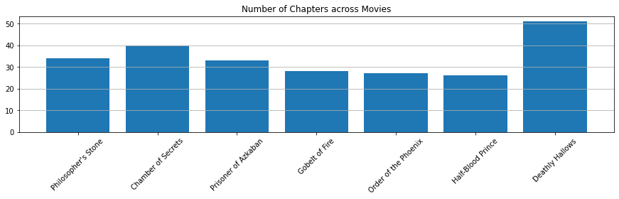

Number of Characters across Movies

characters = []
for i in range(7):
    n_characters = hp_dict[i+1].character.nunique()
    characters.append(n_characters)
    
plt.figure(figsize=(15, 3))
plt.bar(range(7), characters)
plt.xticks([x for x in range(7)], labels=titles, rotation=45)
plt.title("Number of Characters across Movies")
plt.grid(axis="y")
plt.show()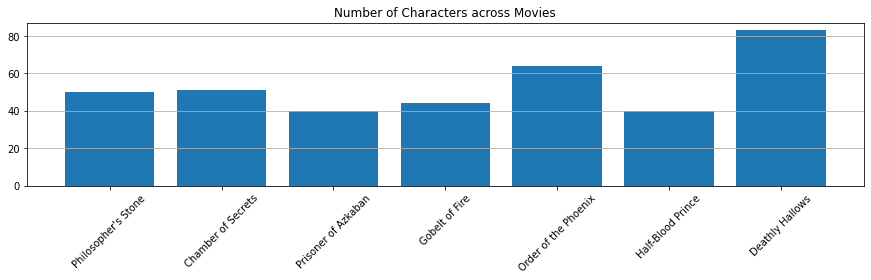

Number of Dialogs across Movies

dialogs = []
for i in range(7):
    n_dialogs = hp_dict[i+1].shape[0]
    dialogs.append(n_dialogs)
    
plt.figure(figsize=(15, 3))
plt.bar(range(7), dialogs)
plt.xticks([x for x in range(7)], labels=titles, rotation=45)
plt.title("Number of Dialogs across Movies")
plt.grid(axis="y")
plt.show()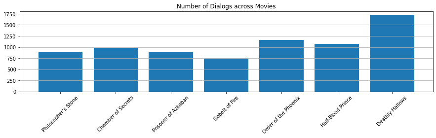

Number of Characters’ Lines

plt.figure(figsize=(15, 10))
for i in range(7):
    plt.subplot(3, 3, i+1)
    character_lines = hp_dict[i+1].groupby("character")["dialog"].count().sort_values()[::-1]
    y = character_lines.index[:10]
    width = character_lines.values[:10]
    plt.barh(y=y[::-1], width=width[::-1])
    plt.title(titles[i])
    plt.grid(axis="x")
plt.tight_layout()
plt.show()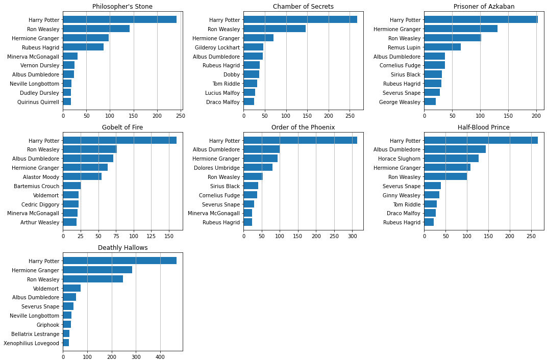

Vocab Size, Total Word, Vocab Ratio

def extract_ngrams(x_raw, 
                   token_pattern=r'\b[A-Za-z][A-Za-z]+\b', 
                   ngram_range=(1, 3), 
                   stop_words=[], 
                   vocab=set()):
    
    # First extract all unigrams by tokenising
    tokenRE = re.compile(token_pattern)
    x_uni = [w for w in tokenRE.findall(str(x_raw).lower(),) if w not in stop_words]
    
    # This is to store the ngrams to be returned
    x = []
    
    if ngram_range[0]==1:
        x = x_uni

    # Generate n-grams from the available unigrams x_uni
    ngrams = []
    for n in range(ngram_range[0], ngram_range[1]+1):

    # Ignore unigrams
        if n==1: continue

        # Pass a list of lists as an argument for zip
        arg_list = [x_uni]+[x_uni[i:] for i in range(1, n)]

        # Extract tuples of n-grams using zip
        x_ngram = list(zip(*arg_list))
        ngrams.append(x_ngram)

    for n in ngrams:
        for t in n:
            x.append(t)

    if len(vocab)>0:
        x = [w for w in x if w in vocab]
        
    return x

def get_vocab(X_raw, 
              ngram_range=(1, 3), 
              min_df=0, 
              keep_topN=0, 
              stop_words=[]):
    
    df = Counter()
    ngram_counts = Counter()
    vocab = set()
    
    # Iterate through each raw text
    for x in X_raw:
        
        x_ngram = extract_ngrams(x, 
                                 ngram_range=ngram_range, 
                                 stop_words=stop_words)
        
        # Update doc and ngram frequencies 
        df.update(list(set(x_ngram)))
        ngram_counts.update(x_ngram)

    # Obtain a vocabulary as a set. 
    # Keep elements with doc frequency > minimum doc freq (min_df)
    # Note that df contains all te
    vocab = set([w for w in df if df[w]>=min_df])
    
    # Keep the top N most freqent 
    if keep_topN > 0:
        vocab = set([w[0] for w in ngram_counts.most_common(keep_topN) 
                     if w[0] in vocab])
    
    return vocab, df, ngram_counts

stop_words = [
    'a','in','on','at','and','or',
    'to', 'the', 'of', 'an', 'by',
    'as', 'is', 'was', 'were', 'been', 'be',
    'are','for', 'this', 'that', 'these', 'those', 'you', 'i', 'if',
    'it', 'he', 'she', 'we', 'they', 'will', 'have', 'has',
    'do', 'did', 'can', 'could', 'who', 'which', 'what',
    'but', 'not', 'there', 'no', 'does', 'not', 'so', 've', 'their',
    'his', 'her', 'they', 'them', 'from', 'with', 'its'
]

Vocab Size

plt.figure(figsize=(15, 3))
vocab_size = []
for i in range(7):
    vocab, df, ngram_counts = get_vocab(hp_dict[i+1]["dialog"], 
                                        ngram_range=(1, 1), 
                                        stop_words=stop_words)
    vocab_size.append(len(vocab))
plt.bar(x=titles, height=vocab_size)
plt.title("Unique Words across Movies")
plt.xticks(rotation=45)
plt.grid(axis="y")
plt.show()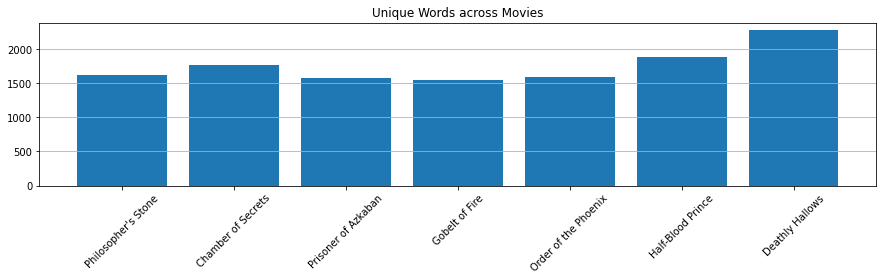

Total Words

token_pattern=r'\b[A-Za-z][A-Za-z]+\b'
tokenRE = re.compile(token_pattern)
hp_lengths = []
for i in range(7):
    length = 0
    for idx in range(len(hp_dict[i+1]["dialog"])):
        x_uni = [w for w in tokenRE.findall(str(hp_dict[i+1].iloc[idx]["dialog"]).lower(),) if w not in stop_words]
        length += len(x_uni)
    hp_lengths.append(length)

plt.figure(figsize=(15, 3))
plt.bar(x=titles, height=hp_lengths)
plt.title("Total Words across Movies")
plt.xticks(rotation=45)
plt.grid(axis="y")
plt.show()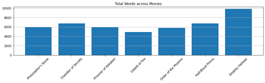

Vocab Ratio

plt.figure(figsize=(15, 3))
plt.bar(x=titles, height=[v/l for v, l in zip(vocab_size, hp_lengths)])
plt.title("Vocab Ratio across Movies")
plt.xticks(rotation=45)
plt.grid(axis="y")
plt.show()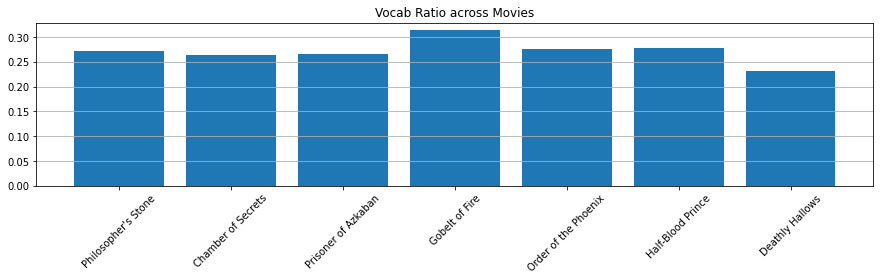

Put it all Together

plt.figure(figsize=(15, 6))
plt.subplot(1, 3, 1)
plt.barh(y=titles[::-1], width=vocab_size[::-1])
plt.title("Unique Words across Movies")
plt.grid(axis="x")
plt.subplot(1, 3, 2)
plt.barh(y=titles[::-1], width=hp_lengths[::-1])
plt.title("Total Words across Movies")
plt.yticks([])
plt.grid(axis="x")
plt.subplot(1, 3, 3)
plt.barh(y=titles[::-1], width=[v/l for v, l in zip(vocab_size[::-1], hp_lengths[::-1])])
plt.title("Vocab Ratio across Movies")
plt.yticks([])
plt.grid(axis="x")
plt.tight_layout()
plt.show()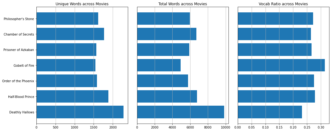

Most Common Words (TF)

plt.figure(figsize=(15, 10))
for i in range(7):
    plt.subplot(3, 3, i+1)
    vocab, df, ngram_counts = get_vocab(hp_dict[i+1]["dialog"], 
                                        ngram_range=(1, 1), 
                                        min_df=0, 
                                        keep_topN=0, 
                                        stop_words=chachedWords)
    y = [ngram[0] for ngram in ngram_counts.most_common(n=10)]
    width = [ngram[1] for ngram in ngram_counts.most_common(n=10)]
    plt.barh(y=y[::-1], width=width[::-1])
    plt.title(titles[i])
    plt.grid(axis="x")
plt.tight_layout()
plt.show()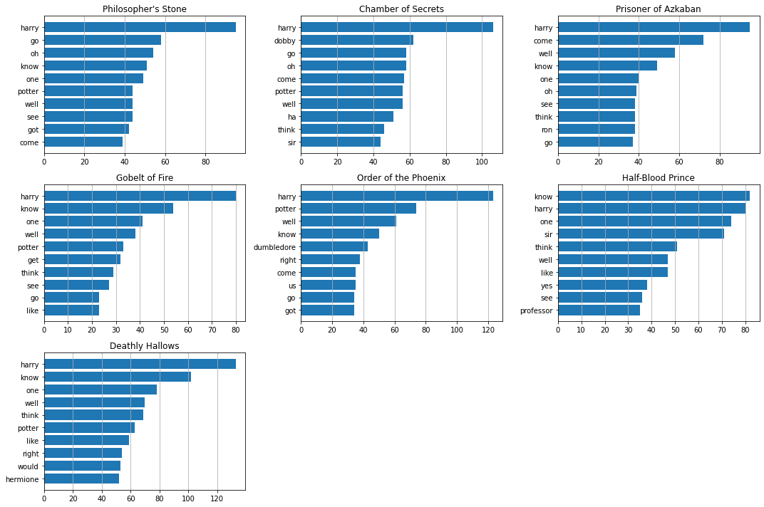

Word Embedding using Word2Vec

Train Word2Vec model with gensim.

from gensim.models import Word2Vec

tokenised_sentence = []
for i in range(7):
    for sentence in hp_dict[i+1]["dialog"]:
        tokenised = extract_ngrams(sentence, 
                                   token_pattern=r'\b[A-Za-z][A-Za-z]+\b', 
                                   ngram_range=(1, 1))
        tokenised_sentence.append(tokenised)
model = Word2Vec(tokenised_sentence, min_count=1, iter=200)

Visualise the word embedding.

from sklearn.decomposition import PCA

character_wv = [
    "harry", "dumbledore", "dobby", "lily", "ron", "snape", "voldemort", 
    "hermione", "potter", "albus", "weasley", "sirius", "james", 
    "gryffindor", "hufflepuff", "ravenclaw", "slytherin"
]
X = model.wv[character_wv]
pca = PCA(n_components=2)
result = pca.fit_transform(X)

plt.figure(figsize=(15, 10))
plt.scatter(result[:, 0], result[:, 1])
plt.xticks([])
plt.yticks([])
for i, character in enumerate(character_wv):
    plt.annotate(character.capitalize(), xy=(result[i, 0], result[i, 1]), fontsize=15)
plt.show()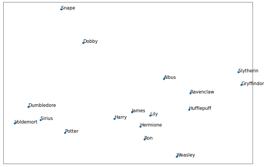

Sentiment Analysis

1. Two sentiment dictionaries:

• Loughran and McDonald Sentiment Word Lists website
• Henry’s (2008) Sentiment Word List paper

2. Negation Rule:

• Any occurrence of negate words (e.g., isn’t, not, never) within three words preceding a positive word will flip that positive word into a negative one.
• Negation check only applies to positive words because Loughran and McDonald (2011) suggest that double negation (i.e., a negate word precedes a negative word) is not common.

Refer from here.

def negated(word):
    """
    Determine if preceding word is a negation word
    """
    if word.lower() in negate:
        return True
    else:
        return False
 
 
def tone_count_with_negation_check(dict_, article, print_result=False):
    """
    Count positive and negative words with negation check. Account for simple negation only for positive words.
    Simple negation is taken to be observations of one of negate words occurring within three words
    preceding a positive words.
    """
    pos_count = 0
    neg_count = 0
 
    pos_words = []
    neg_words = []
 
    input_words = re.findall(r'\b([a-zA-Z]+n\'t|[a-zA-Z]+\'s|[a-zA-Z]+)\b', article.lower())
 
    word_count = len(input_words)
 
    for i in range(0, word_count):
        if input_words[i] in dict_['Negative']:
            neg_count += 1
            neg_words.append(input_words[i])
        if input_words[i] in dict_['Positive']:
            if i >= 3:
                if negated(input_words[i - 1]) or negated(input_words[i - 2]) or negated(input_words[i - 3]):
                    neg_count += 1
                    neg_words.append(input_words[i] + ' (with negation)')
                else:
                    pos_count += 1
                    pos_words.append(input_words[i])
            elif i == 2:
                if negated(input_words[i - 1]) or negated(input_words[i - 2]):
                    neg_count += 1
                    neg_words.append(input_words[i] + ' (with negation)')
                else:
                    pos_count += 1
                    pos_words.append(input_words[i])
            elif i == 1:
                if negated(input_words[i - 1]):
                    neg_count += 1
                    neg_words.append(input_words[i] + ' (with negation)')
                else:
                    pos_count += 1
                    pos_words.append(input_words[i])
            elif i == 0:
                pos_count += 1
                pos_words.append(input_words[i])
 
    if print_result:
        print('The results with negation check:', end='\n\n')
        print('The # of positive words:', pos_count)
        print('The # of negative words:', neg_count)
        print('The list of found positive words:', pos_words)
        print('The list of found negative words:', neg_words)
        print('\n', end='')
 
    results = [word_count, pos_count, neg_count, pos_words, neg_words]
 
    return results

Calculate the Sentiment Score

for i in range(7):
    features = ["word_count", "pos_count", "neg_count", "pos_words", "neg_words"]
    hp_dict[i+1]["dialog"] = hp_dict[i+1]["dialog"].map(str)
    hp_dict[i+1][features] = hp_dict[i+1]["dialog"].apply(lambda x: pd.Series(tone_count_with_negation_check(lmdict, x)))

plt.figure(figsize=(15, 10))
for i in range(7):
    plt.subplot(4, 2, i+1)
    df = hp_dict[i+1].groupby("chapter").agg({"pos_count": "sum", "neg_count": "sum"})
    plt.plot(df["pos_count"], label="positive")
    plt.plot(df["neg_count"], label="negative")
    plt.title(f"{titles[i]}\nSentiment across {chapters[i]} Chapters")
    plt.xticks([])
    plt.legend(loc="upper right")
    plt.grid()
plt.tight_layout()
plt.show()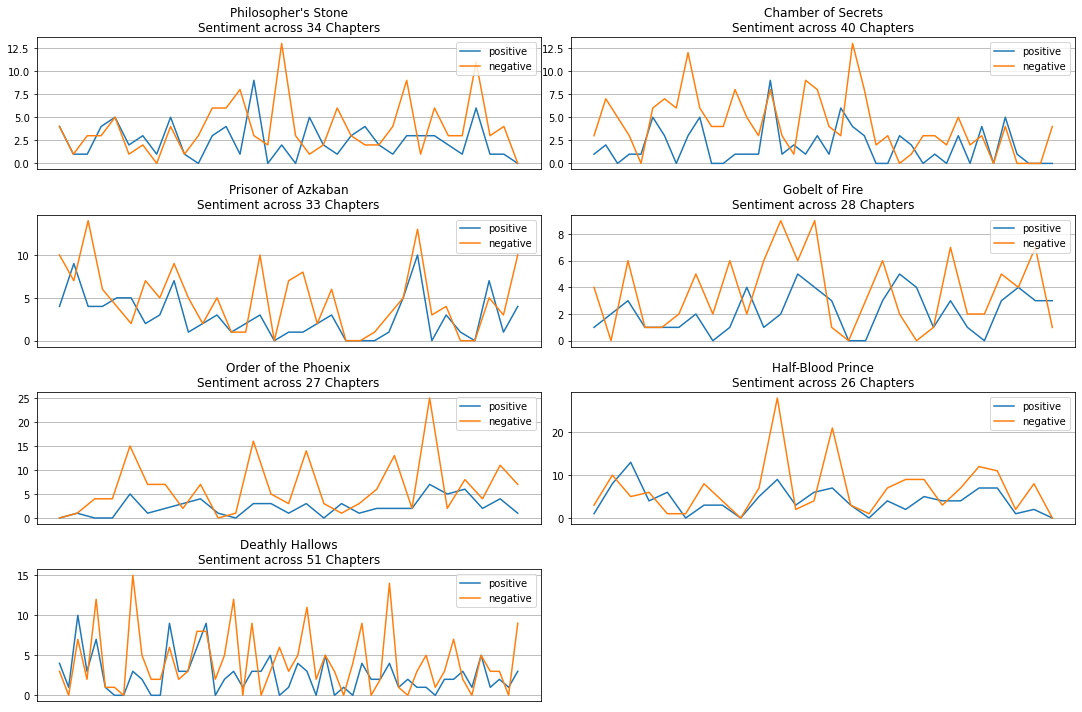

Sentiment across Movies

How does sentiment usually change of the course of one school year? I compute the s-score by:

plt.figure(figsize=(15, 8))
EPSILON = 1e-8
colors = sns.color_palette("hls", 7)
for i in range(7):
    plt.subplot(4, 2, i+1)
    df = hp_dict[i+1].groupby("chapter").agg({"pos_count": "sum", "neg_count": "sum"})
    s_score = [(x-y+EPSILON)/(x+y+EPSILON) for x, y in zip(df["pos_count"], df["neg_count"])]
    plt.plot(s_score, color=colors[i])
    plt.title(titles[i])
    plt.xticks([x for x in range(0, len(s_score), 5)])
    plt.grid()
plt.tight_layout()
plt.show()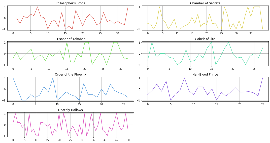

plt.figure(figsize=(15, 6))
cum_sum = 0
EPSILON = 1e-8
for i in range(7):
    df = hp_dict[i+1].groupby("chapter").agg({"pos_count": "sum", "neg_count": "sum"})
    s_score = [(x-y+EPSILON)/(x+y+EPSILON) for x, y in zip(df["pos_count"], df["neg_count"])]
    plt.plot(list(range(cum_sum, cum_sum+len(s_score))), s_score, label=titles[i])
    cum_sum += len(s_score)
    plt.title("Sentiment across Movies")
    plt.xticks([])
    plt.legend(loc="upper right")
plt.grid()
plt.show()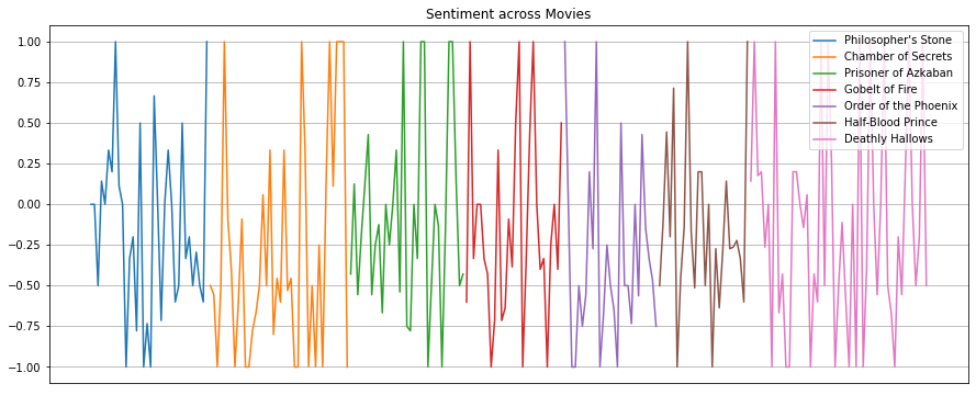

plt.figure(figsize=(15, 8))
EPSILON = 1e-8
colors = sns.color_palette("hls", 7)
for i in range(7):
    plt.subplot(4, 2, i+1)
    df = hp_dict[i+1]
    pos_count_ma = df["pos_count"].rolling(20).mean()
    plt.plot(range(len(pos_count_ma)), pos_count_ma, color=colors[i])
    plt.title(titles[i])
    plt.xticks([])
    plt.grid()
plt.tight_layout()
plt.show()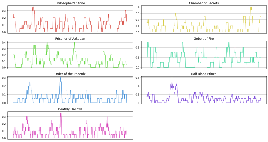

plt.figure(figsize=(15, 8))
EPSILON = 1e-8
colors = sns.color_palette("hls", 7)
for i in range(7):
    plt.subplot(4, 2, i+1)
    df = hp_dict[i+1]
    neg_count_ma = df["neg_count"].rolling(20).mean()
    plt.plot(range(len(neg_count_ma)), neg_count_ma, color=colors[i])
    plt.title(titles[i])
    plt.xticks([])
    plt.grid()
plt.tight_layout()
plt.show()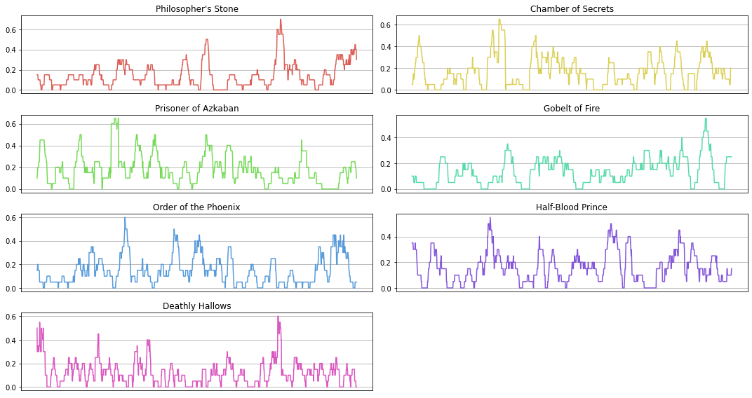

Sentiment for 3 Main Characters

plt.figure(figsize=(15, 10))
character_list = ["Harry Potter", "Hermione Granger", "Ron Weasley"]
s_scores = []
for i, char in enumerate(character_list):
    plt.subplot(3, 1, i+1)
    
    pos_count_average, neg_count_average = [], []
    for i in range(7):
        df = hp_dict[i+1].loc[hp_dict[i+1].character==char]
        pos_mean = sum(df.pos_count) / df.shape[0]
        neg_mean = sum(df.neg_count) / df.shape[0]
        pos_count_average.append(pos_mean)
        neg_count_average.append(neg_mean)
    
    s_score = [(x-y)/(x+y) for x, y in zip(pos_count_average, neg_count_average)]
    s_scores.append(s_score)
        
    plt.plot(pos_count_average, label="positive average")
    plt.plot(neg_count_average, label="negative average")
    plt.title(f"{char}'s Sentiment Average across Movies")
    if char == character_list[-1]:
        plt.xticks([x for x in range(7)], labels=titles, rotation=45)
    else:
        plt.xticks(ticks=[x for x in range(7)], labels=[])
    plt.legend()
    plt.grid(axis="both")
plt.tight_layout()
plt.show()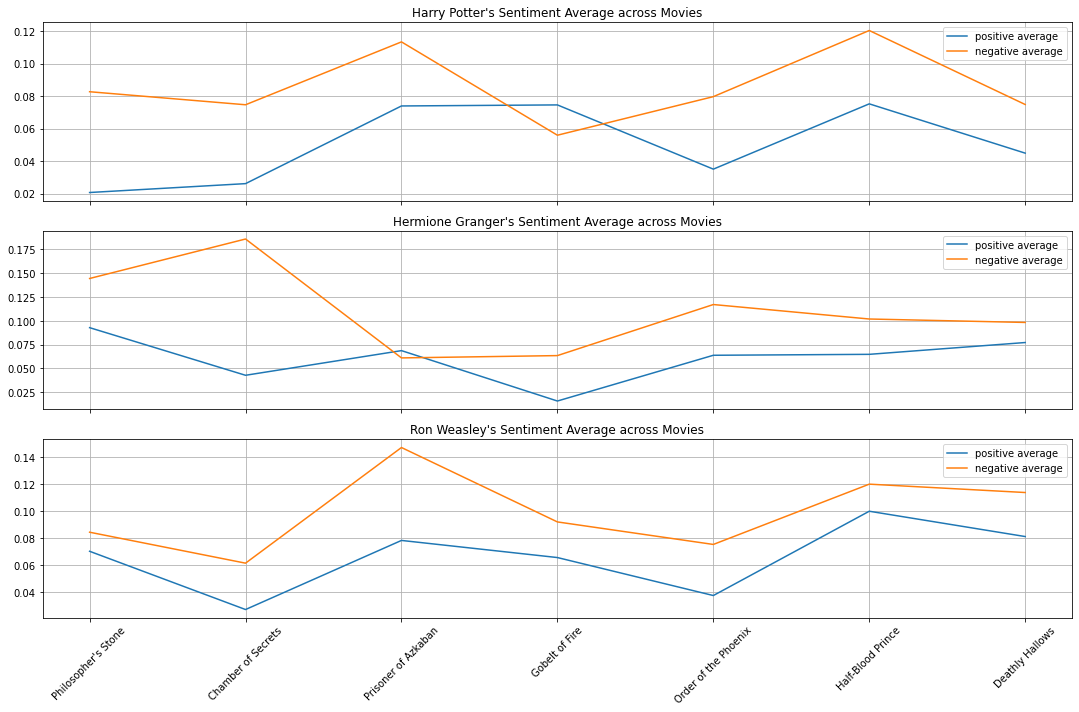

plt.figure(figsize=(15, 6))
for i, char in enumerate(character_list):
    plt.plot(s_scores[i], label=char)
plt.legend(loc="upper right")
plt.title("Sentiment of Three Main Characters across Movies")
plt.xticks([x for x in range(7)], labels=titles, rotation=45)
plt.grid()
plt.show()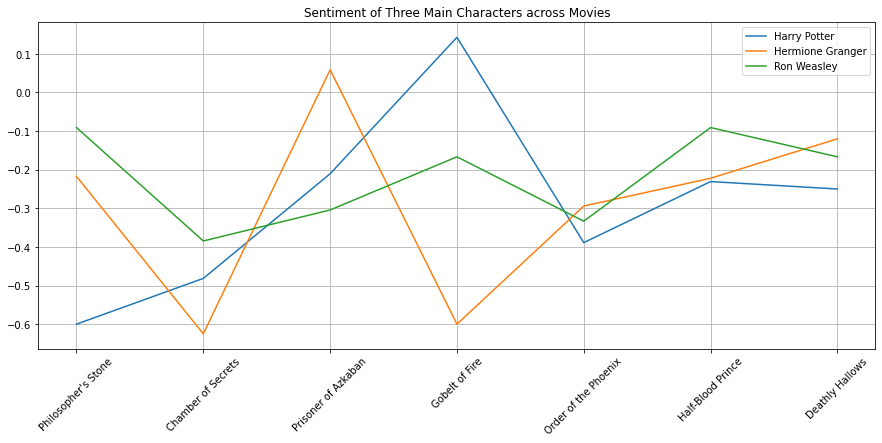

TFIDF for Sentiment

for i in range(7):
    for idx, row in hp_dict[i+1].iterrows():
        if (row["pos_count"] - row["neg_count"]) > 0:
            hp_dict[i+1].loc[idx, "polarity"] = "positive"
        elif (row["pos_count"] - row["neg_count"]) == 0:
            hp_dict[i+1].loc[idx, "polarity"] = "neutral"
        elif (row["pos_count"] - row["neg_count"]) < 0:
            hp_dict[i+1].loc[idx, "polarity"] = "negative"

Build the function for visualisation.

# Refer from https://buhrmann.github.io/tfidf-analysis.html

def top_tfidf_feats(row, features, top_n=25):
    ''' Get top n tfidf values in row and return them with their corresponding feature names.'''
    topn_ids = np.argsort(row)[::-1][:top_n]
    top_feats = [(features[i], row[i]) for i in topn_ids]
    df = pd.DataFrame(top_feats)
    df.columns = ['feature', 'tfidf']
    return df

def top_feats_in_doc(Xtr, features, row_id, top_n=25):
    ''' Top tfidf features in specific document (matrix row)'''
    row = np.squeeze(Xtr[row_id].toarray())
    return top_tfidf_feats(row, features, top_n)

def top_mean_feats(Xtr, features, grp_ids=None, min_tfidf=0.1, top_n=25):
    ''' Return the top n features that on average are most important amongst documents in rows
        indentified by indices in grp_ids.'''
    if grp_ids:
        D = Xtr[grp_ids].toarray()
    else:
        D = Xtr.toarray()

    D[D < min_tfidf] = 0
    tfidf_means = np.mean(D, axis=0)
    return top_tfidf_feats(tfidf_means, features, top_n)

def top_feats_by_class(Xtr, y, features, min_tfidf=0.1, top_n=25):
    ''' Return a list of dfs, where each df holds top_n features and their mean tfidf value
        calculated across documents with the same class label. '''
    dfs = []
    labels = np.unique(y)
    for label in labels:
        ids = np.where(y==label)
        feats_df = top_mean_feats(Xtr, features, ids, min_tfidf=min_tfidf, top_n=top_n)
        feats_df.label = label
        dfs.append(feats_df)
    return dfs

def plot_tfidf_classfeats_h(dfs):
    ''' Plot the data frames returned by the function plot_tfidf_classfeats(). '''
    fig = plt.figure(figsize=(15, 9), facecolor="w")
    x = np.arange(len(dfs[0]))
    for i, df in enumerate(dfs):
        ax = fig.add_subplot(1, len(dfs), i+1)
        ax.spines["top"].set_visible(False)
        ax.spines["right"].set_visible(False)
        ax.set_frame_on(False)
        ax.get_xaxis().tick_bottom()
        ax.get_yaxis().tick_left()
        ax.set_xlabel("Mean Tf-Idf Score", labelpad=16, fontsize=14)
        ax.set_title("label = " + str(df.label), fontsize=16)
        ax.ticklabel_format(axis='x', style='sci', scilimits=(-2,2))
        ax.barh(x, df.tfidf, align='center', color='#3F5D7D')
        ax.set_yticks(x)
        ax.set_ylim([-1, x[-1]+1])
        yticks = ax.set_yticklabels(df.feature)
        plt.subplots_adjust(bottom=0.09, right=0.97, left=0.15, top=0.95, wspace=0.52)
    plt.show()

You can change the parameter episode to see what the difference is.

from sklearn.feature_extraction.text import TfidfVectorizer

episode = 1

vec_pipe = TfidfVectorizer(ngram_range=(1, 1), max_features=1000, stop_words=chachedWords)
Xtr = vec_pipe.fit_transform(pd.Series(hp_dict[episode]["dialog"]))
features = vec_pipe.get_feature_names()

dfs = top_feats_by_class(Xtr, hp_dict[episode]["polarity"], features, top_n=10)
plot_tfidf_classfeats_h(dfs)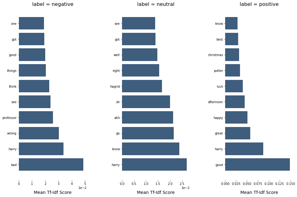

You can also visualise bigram.

vec_pipe = TfidfVectorizer(ngram_range=(2, 2), max_features=1000, stop_words=chachedWords)
Xtr = vec_pipe.fit_transform(pd.Series(hp_dict[episode]["dialog"]))
features = vec_pipe.get_feature_names()

dfs = top_feats_by_class(Xtr, hp_dict[episode]["polarity"], features, top_n=10)
plot_tfidf_classfeats_h(dfs)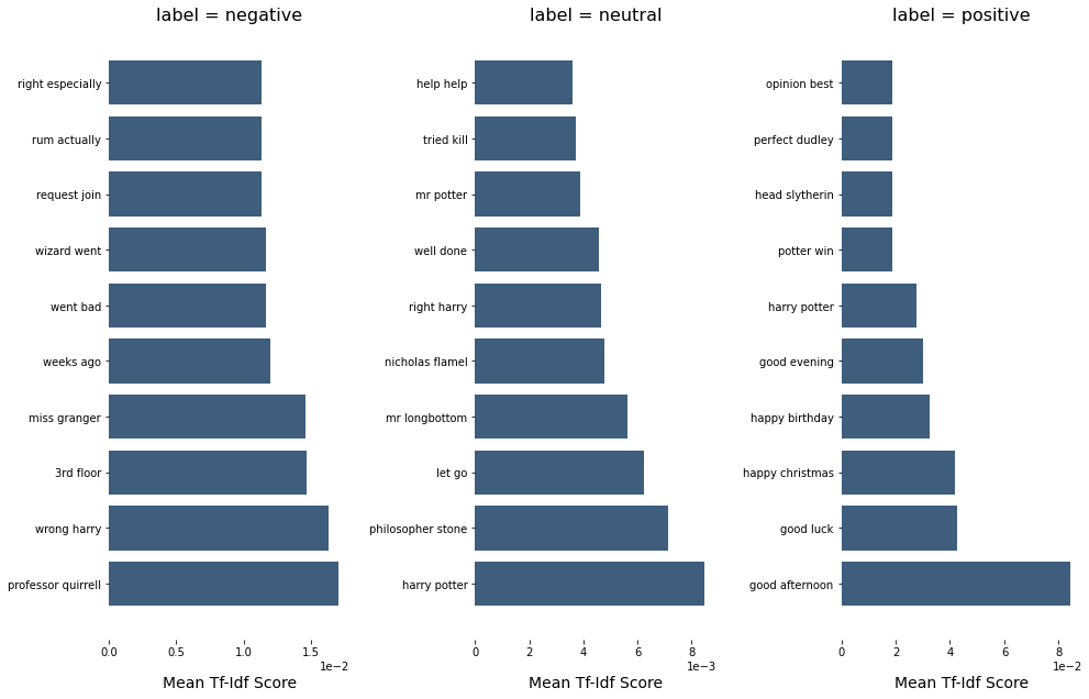

NRC Emotional Lexicon

This is the NRC Emotional Lexicon: “The NRC Emotion Lexicon is a list of English words and their associations with eight basic emotions (anger, fear, anticipation, trust, surprise, sadness, joy, and disgust) and two sentiments (negative and positive). The annotations were manually done by crowdsourcing.”

filepath = r"NRC-Emotion-Lexicon-Wordlevel-v0.92.txt"
emolex_df = pd.read_csv(filepath,  names=["word", "emotion", "association"], skiprows=45, sep='\t')

# Reshape the data in order to look at it a slightly different way
emolex_words = emolex_df.pivot(index='word', columns='emotion', values='association').fillna(0).reset_index()
emolex_words = emolex_words.dropna()

First, tokenise all the dialog in each episode.

tokenised_sentence_per_episode = []
for i in range(7):
    tokenised_sentence_per_dialog = []
    for sentence in hp_dict[i+1]["dialog"]:
        tokenised = extract_ngrams(sentence, 
                                   token_pattern=r'\b[A-Za-z][A-Za-z]+\b', 
                                   ngram_range=(1, 1))
        tokenised_sentence_per_dialog.append(tokenised)
    tokenised_sentence_per_episode.append(tokenised_sentence_per_dialog)

Get the emotion score for each dialog, and calculate the mean of every score.

emotion_dict = {}
for idx, episode in enumerate(tokenised_sentence_per_episode):
    emotion_arr = []
    for dialog in episode:
        dialog = [d for d in dialog if d in emolex_words.word.tolist()]
        arr = emolex_words.loc[emolex_words['word'].isin(dialog)].iloc[:, 1:].mean(axis=0).values
        emotion_arr.append(arr)
    emotion_df = pd.DataFrame(np.array(emotion_arr)).fillna(0.0)
    emotion_df.columns = ["anger", "anticipation", "disgust", "fear", "joy", 
                          "negative", "positive", "sadness", "surprise", "trust"]
    emotion_dict[idx+1] = emotion_df

for i in range(7):
    hp_dict[i+1] = pd.concat([hp_dict[i+1], emotion_dict[i+1]], axis=1)

Visualise Emotion across Chapters

plt.figure(figsize=(15, 15))
for i in range(7):
    plt.subplot(4, 2, i+1)
    df = hp_dict[i+1].groupby("chapter").agg({"anger": "mean", 
                                              "anticipation": "mean", 
                                              "disgust": "mean", 
                                              "fear": "mean", 
                                              "joy": "mean", 
                                              "negative": "mean", 
                                              "positive": "mean", 
                                              "sadness": "mean", 
                                              "surprise": "mean", 
                                              "trust": "mean"})
    plt.plot(df["anger"], label="anger")
    plt.plot(df["anticipation"], label="anticipation")
    plt.plot(df["disgust"], label="disgust")
    plt.plot(df["fear"], label="fear")
    plt.plot(df["joy"], label="joy")
    plt.plot(df["negative"], label="negative")
    plt.plot(df["positive"], label="positive")
    plt.plot(df["sadness"], label="sadness")
    plt.plot(df["surprise"], label="surprise")
    plt.plot(df["trust"], label="trust")
    plt.title(f"{titles[i]}\nEmotion across {chapters[i]} Chapters")
    plt.xticks([])
    plt.legend(loc="upper right")
    plt.grid()
plt.tight_layout()
plt.show()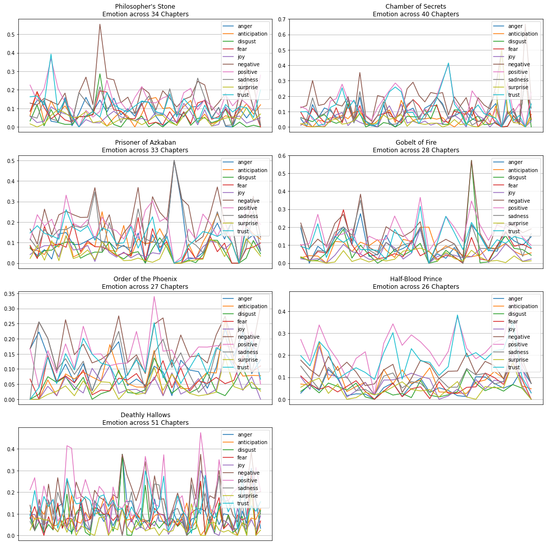

plt.figure(figsize=(15, 15))
emotions = ["anger", "anticipation", "disgust", "fear", "joy", "negative", "positive", "sadness", "surprise", "trust"]
for idx, emotion in enumerate(emotions):
    plt.subplot(5, 2, idx+1)
    cum = 0
    for i in range(7):
        df = hp_dict[i+1].groupby("chapter").agg({emotion: "mean"})
        plt.plot(range(cum, cum+len(df)), df[emotion], label=titles[i])
        plt.xticks([])
        cum += len(df)
    plt.title(emotion.capitalize())
    plt.legend(loc="upper right")
    plt.grid()
plt.tight_layout()
plt.show()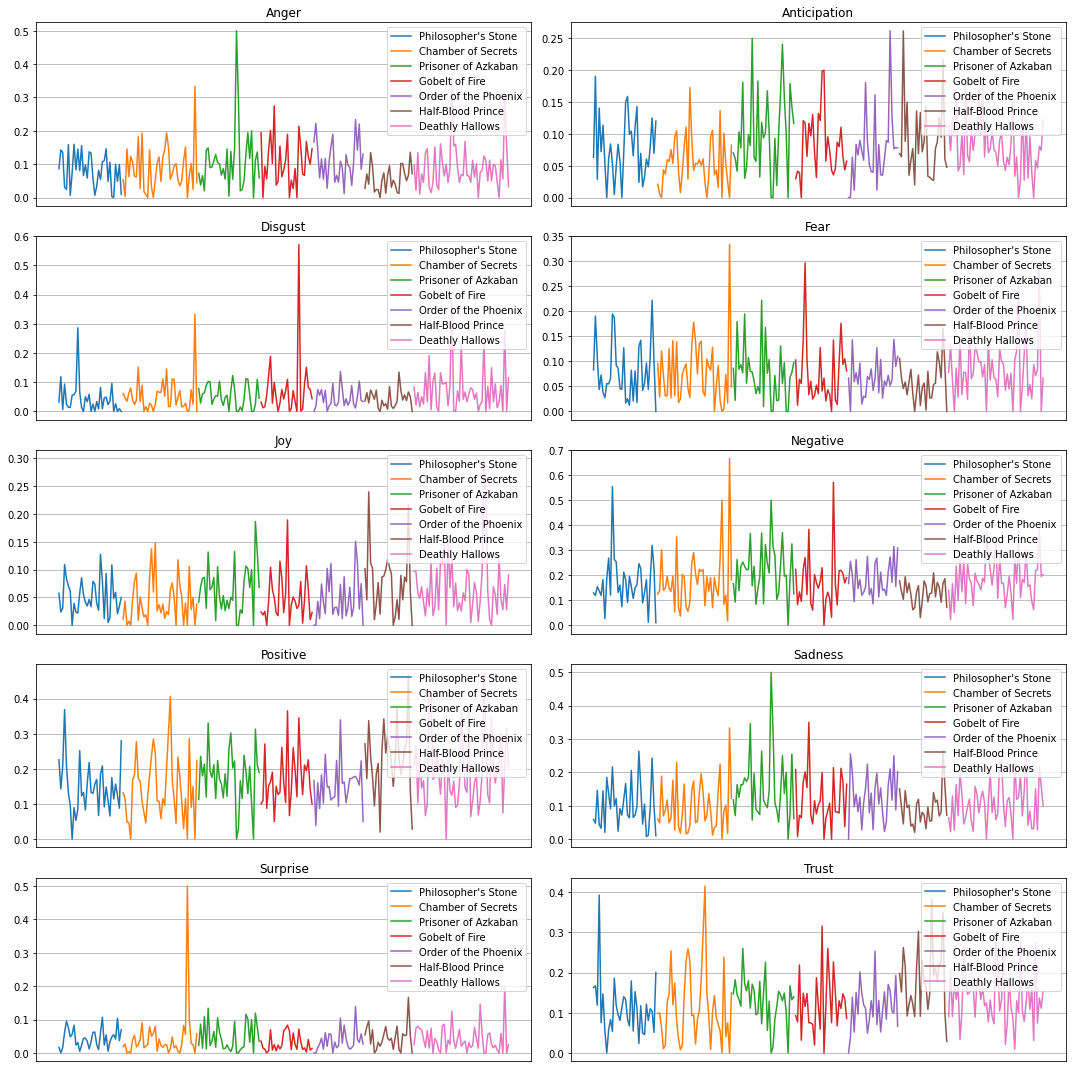

Conclusion

I was really excited to dive into this NLP side project for Harry Potter. We can find out more about how we can use the magic of NLP. I put the jupyter notebook over here, you can run it by yourself.

Reference

1. https://laptrinhx.com/basic-nlp-on-the-texts-of-harry-potter-sentiment-analysis-864442763/
2. https://rpubs.com/Siebelm/Harry_Potter_2
3. https://www.kaggle.com/asterol/harry-potter-and-the-sorcecers-stone-nlp-analysis
4. https://towardsdatascience.com/basic-nlp-on-the-texts-of-harry-potter-sentiment-analysis-1b474b13651d
5. https://siebelm.github.io/Harry_Potter_1/
6. http://jonathansoma.com/lede/algorithms-2017/classes/more-text-analysis/nrc-emotional-lexicon/
7. http://saifmohammad.com/WebPages/AccessResource.htm
8. https://github.com/NBrisbon/Silmarillion-NLP/blob/master/Sentiment_Visualizations.ipynb