Predicting Stock Price using LSTM

Introduction

This article tends to build a model that predicts stock price in the best way possible. This is an example of how you can use Long Short-Term Memory (LSTM) Neural Network on some real-world time series data with PyTorch. Hopefully, there are much better models that forecast the price of the stock.

Load Data

Load the package.

import torch
import torch.nn as nn
import torch.optim as optim
import torch.nn.functional as F
import numpy as np
import pandas as pd
import yfinance as yf
import matplotlib.pyplot as plt
import seaborn as sns
from sklearn.preprocessing import MinMaxScaler

Load the data using Yahoo Finance API.

stock = yf.download(tickers="DIS", progress=False)
stock = stock.loc["2015":]

Preprocessing

Split the data. We have 955 training data, 319 validation data, and 319 test data.

stock_close = stock["Close"]

t_v_split = int(0.6*len(stock_close))
v_t_split = int(0.8*len(stock_close))
train_data, valid_data, test_data = stock_close[:t_v_split], stock_close[t_v_split:v_t_split], stock_close[v_t_split:]

Scale the data.

scaler = MinMaxScaler()
train_data = scaler.fit_transform(np.expand_dims(train_data, axis=1))
valid_data = scaler.transform(np.expand_dims(valid_data, axis=1))
test_data = scaler.transform(np.expand_dims(test_data, axis=1))

def sliding_windows(data, seq_length):
    xs, ys = [], []
    
    for i in range(len(data)-seq_length-1):
        x = data[i:(i+seq_length)]
        y = data[i+seq_length]
        xs.append(x)
        ys.append(y)
        
    return np.array(xs), np.array(ys)

For each example contains 64 data points of history and a label for the real value that our model needs to predict.

SEQ_LENGTH = 64

X_train, y_train = sliding_windows(train_data, SEQ_LENGTH)
X_valid, y_valid = sliding_windows(valid_data, SEQ_LENGTH)
X_test, y_test = sliding_windows(test_data, SEQ_LENGTH)

X_train = torch.from_numpy(X_train).float()
X_valid = torch.from_numpy(X_valid).float()
X_test = torch.from_numpy(X_test).float()

y_train = torch.from_numpy(y_train).float()
y_valid = torch.from_numpy(y_valid).float()
y_test = torch.from_numpy(y_test).float()

Long Short-Term Memory

Long short-term memory (LSTM) is an artificial recurrent neural network (RNN) architecture used in the field of deep learning. Unlike standard feedforward neural networks, LSTM has feedback connections. It can not only process single data points (such as images), but also entire sequences of data (such as speech or video).

The compact forms of the equations for the forward pass of an LSTM unit are:

where the initial values are and and the operator denotes the Hadamard product (element-wise product). The subscript indexes the time step.

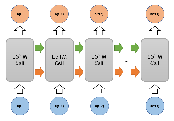
Time Series Structure of LSTM

One of the most common diagram of LSTM showed below. Personally, I find this diagram very misleading for beginners, and there are two issues which should be aware of.

1. This is a diagram of the logic of the LSTM, but it doesn’t actually look like this.
2. This is a diagram of the forward and backward inputs and outputs in the time series, not the actual situation at the same time.

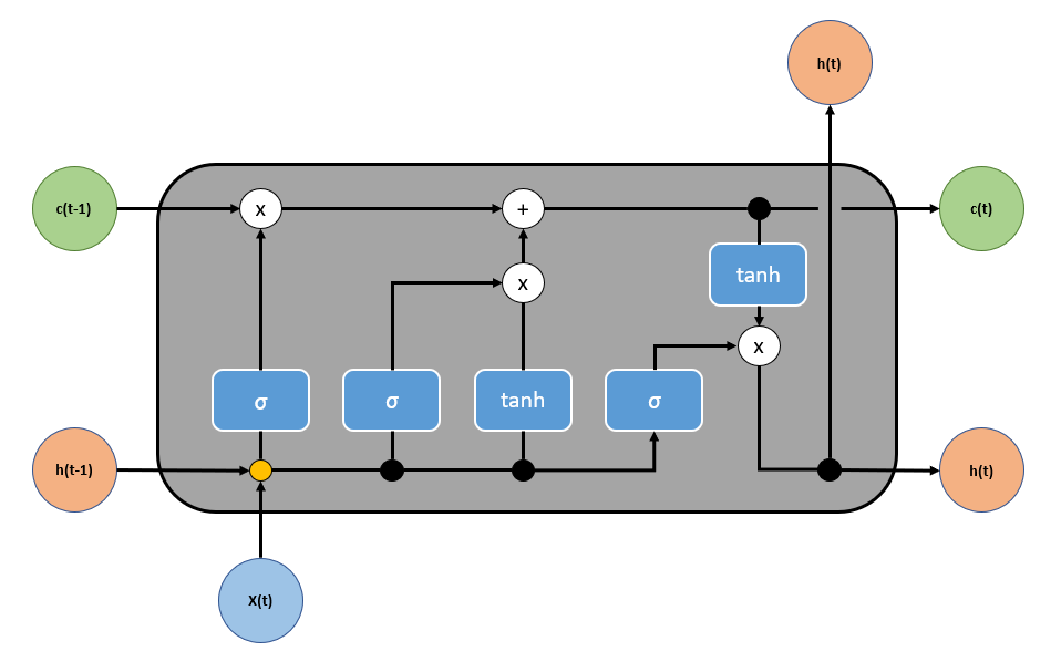
Actual Structure of LSTM

1. This LSTM cell computes the current x(t), h(t) and c(t) three vectors to obtain the output and state of the current moment.
2. Here the value of input x(t) is the size of the word embedding vector. disregard batch size, that is, batch size equals to 1)

What’s inside LSTM?

Parameters in the below graph:

1. One hidden layer
2. Vector length of X is 6
3. Number of unit is 128
4. Batch size of 1

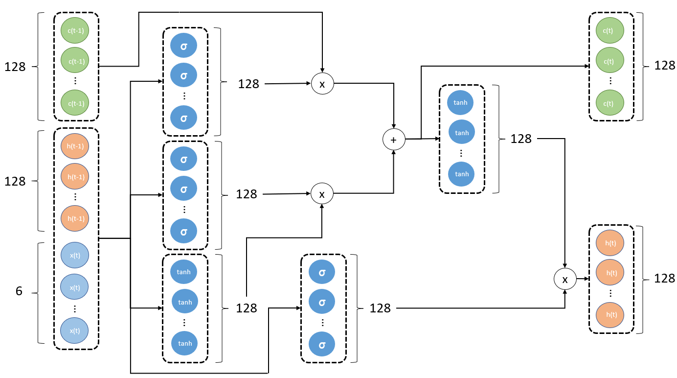
This diagram is the real physical architecture using neural networks to implement LSTM. The following points should be noted:

1. The number of neurons in each layer is the size of unit_num.
2. The output vector h(t) and state vector c(t) length of each cell is also the size of unit_num.

You can also look at this website to see a similar explanation.

Build Model

We’ll excapsulate the complexity of our model into a class that extends from torch.nn.Module.

class StockPredictor(nn.Module):
    
    def __init__(self, input_size, hidden_size, num_layers, seq_length, dropout):
        super(StockPredictor, self).__init__()
        self.input_size = input_size
        self.hidden_size = hidden_size
        self.num_layers = num_layers
        self.seq_length = seq_length
        self.dropout = dropout
        
        self.lstm = nn.LSTM(input_size=input_size, 
                            hidden_size=hidden_size, 
                            num_layers=num_layers, 
                            dropout=dropout)
        self.linear = nn.Linear(in_features=hidden_size, out_features=1)
        
    def reset_hidden_state(self, device):
        self.hidden = (
            torch.zeros(self.num_layers, self.seq_length, self.hidden_size).to(device), 
            torch.zeros(self.num_layers, self.seq_length, self.hidden_size).to(device)
        )
        
    def forward(self, input_):
        lstm_out, self.hidden = self.lstm(input_.view(len(input_), self.seq_length, -1), self.hidden)
        y_pred = self.linear(lstm_out.view(self.seq_length, len(input_), self.hidden_size)[-1])
        return y_pred

Train a Model

Build a helper function for the training of our model.

def train_model(model, device, train_data, train_labels, valid_data=None, valid_labels=None, epochs=10):
    loss_fn = nn.MSELoss(reduction="sum").to(device)
    optimiser = optim.Adam(model.parameters(), lr=1e-3, weight_decay=1e-4)
    train_history = np.zeros(EPOCHS)
    valid_history = np.zeros(EPOCHS)
    
    for epoch in range(epochs):
        model.reset_hidden_state(device)
        y_pred = model(train_data.to(device))
        loss = loss_fn(y_pred.float(), train_labels.to(device))
        if valid_data is not None:
            with torch.no_grad():
                y_valid_pred = model(valid_data.to(device))
                valid_loss = loss_fn(y_valid_pred.float(), valid_labels.to(device))
            valid_history[epoch] = valid_loss.item()
            print(f"Epoch {epoch} Train Loss: {loss.item()} Valid Loss: {valid_loss.item()}")
        else:
            print(f"Epoch {epoch} Train Loss: {loss.item()}")
        train_history[epoch] = loss.item()
        optimiser.zero_grad()
        loss.backward()
        optimiser.step()
    return model.eval(), train_history, valid_history

Let’s create an instance of our model and train it.

device = torch.device("cuda" if torch.cuda.is_available() else "cpu")
model = StockPredictor(input_size=1, hidden_size=64, num_layers=2, seq_length=SEQ_LENGTH, dropout=0.25)
model.to(device)

EPOCHS = 20
model, train_history, valid_history = train_model(
	model, 
	device, 
	X_train, 
	y_train, 
	X_valid, 
	y_valid, 
	EPOCHS
)

---

Epoch 0 Train Loss: 342.94207763671875 Valid Loss: 560.39892578125
Epoch 1 Train Loss: 315.7298583984375 Valid Loss: 539.568359375
Epoch 2 Train Loss: 289.62628173828125 Valid Loss: 519.0243530273438
Epoch 3 Train Loss: 264.38861083984375 Valid Loss: 497.4339904785156
Epoch 4 Train Loss: 239.2693328857422 Valid Loss: 476.92999267578125
Epoch 5 Train Loss: 214.5585174560547 Valid Loss: 455.1669921875
Epoch 6 Train Loss: 189.5911865234375 Valid Loss: 432.6599426269531
Epoch 7 Train Loss: 164.21170043945312 Valid Loss: 406.616455078125
Epoch 8 Train Loss: 138.76486206054688 Valid Loss: 379.9129943847656
Epoch 9 Train Loss: 112.80253601074219 Valid Loss: 350.98260498046875
Epoch 10 Train Loss: 87.68815612792969 Valid Loss: 317.3212585449219
Epoch 11 Train Loss: 65.24786376953125 Valid Loss: 280.55157470703125
Epoch 12 Train Loss: 46.86219024658203 Valid Loss: 237.37155151367188
Epoch 13 Train Loss: 38.28335189819336 Valid Loss: 193.4661865234375
Epoch 14 Train Loss: 46.59754943847656 Valid Loss: 150.02650451660156
Epoch 15 Train Loss: 63.70148468017578 Valid Loss: 124.49668884277344
Epoch 16 Train Loss: 70.30477905273438 Valid Loss: 115.31311798095703
Epoch 17 Train Loss: 63.82952880859375 Valid Loss: 125.69139099121094
Epoch 18 Train Loss: 54.24039840698242 Valid Loss: 137.96578979492188
Epoch 19 Train Loss: 45.09291076660156 Valid Loss: 155.43263244628906

Let’s have a look at the train and valid loss.

plt.figure(figsize=(15, 6))
plt.plot(range(EPOCHS), train_history, label="train loss")
plt.plot(range(EPOCHS), valid_history, label="valid loss")
plt.grid()
plt.legend()
plt.show()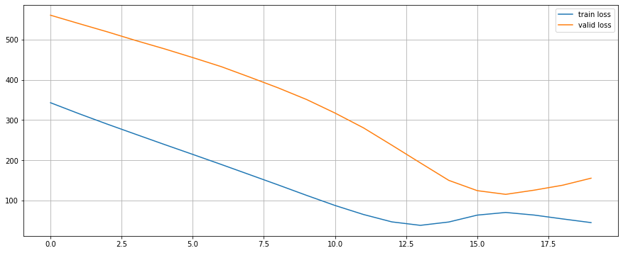

Predict the Price

Our model can predict only a single day in the future. We’ll employ a simple strategy to overcome this limitation. Use predicted values as input for predicting the next days.

with torch.no_grad():
    test_seq = X_test[:1]
    preds = []
    for _ in range(len(X_test)):
        y_test_pred = model(test_seq.to(device))
        pred = torch.flatten(y_test_pred).item()
        preds.append(pred)
        new_seq = test_seq.numpy().flatten()
        new_seq = np.append(new_seq, [pred])
        new_seq = new_seq[1:]
        test_seq = torch.as_tensor(new_seq).view(1, SEQ_LENGTH, 1).float()

Reverse the scaling of the test data and the model predicitons.

true_cases = scaler.inverse_transform(
    np.expand_dims(y_test.flatten().numpy(), axis=0)
).flatten()

predict_cases = scaler.inverse_transform(
    np.expand_dims(preds, axis=0)
).flatten()

Visualise the result.

plt.figure(figsize=(15, 6))
plt.plot(
    stock.index[:len(train_data)], 
    scaler.inverse_transform(train_data).flatten(), 
    label="Historical Close Price (Train)"
)
plt.plot(
    stock.index[len(train_data):len(train_data)+len(valid_data)], 
    scaler.inverse_transform(valid_data).flatten(), 
    label="Historical Close Price (Valid)"
)
plt.plot(
    stock.index[len(train_data)+len(valid_data):len(train_data)+len(valid_data)+len(true_cases)], 
    true_cases, 
    label="Groud Truth Price"
)
plt.plot(
    stock.index[len(train_data)+len(valid_data):len(train_data)+len(valid_data)+len(predict_cases)], 
    predict_cases, 
    label="Predicted Price"
)
plt.grid()
plt.legend()
plt.show()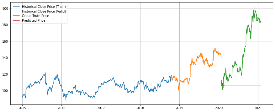

Conclusion

We’ve learned how to use PyTorch to create a LSTM that works with time series data. The model performance does not generalise well at all, but this is as expected.

Reference

1. https://www.youtube.com/watch?v=8A6TEjG2DNw&t=2858s
2. https://www.youtube.com/watch?v=PuZY9q-aKLw&t=5s
3. https://en.wikipedia.org/wiki/Long_short-term_memory