Introduction to Ordinary Least Squares

Introduction

In empirical finance and many other domains, linear regression and the closely related linear prediction theory are commonly used statistical methods. Because of the wide range of applications, basic linear regression courses normally concentrate on the mathematically simplest scenario, which can be used in a variety of other applications.

Ordinary least squares (OLS)

A linear regression model relates the output (or response) to input (or predictor) variables , which are also called regressors, via

where the are unobservable random errors that are assumed to have zero means. The coefficients are unknown parameters that have to be estimated from the observed input-output vectors.

To fit a regression model to the observed data, the method of least squares chooses to minimise the residual sum of squares (RSS).

Setting to 0 the partial derivative of RSS with respect to yields linear equations, whose solution gives the OLS estimates. The regression model can be written in matrix form as

The vector of least squares estimates of the is given by

Using this matrix notation, RSS can be written as

Statistical Properties of OLS Estimates

1. are nonrandom constants and has full rank p, where .
2. are unobserved random disturbances with
3. and for
4. are independent , where denotes the normal distribution with mean and variance .

Case Study

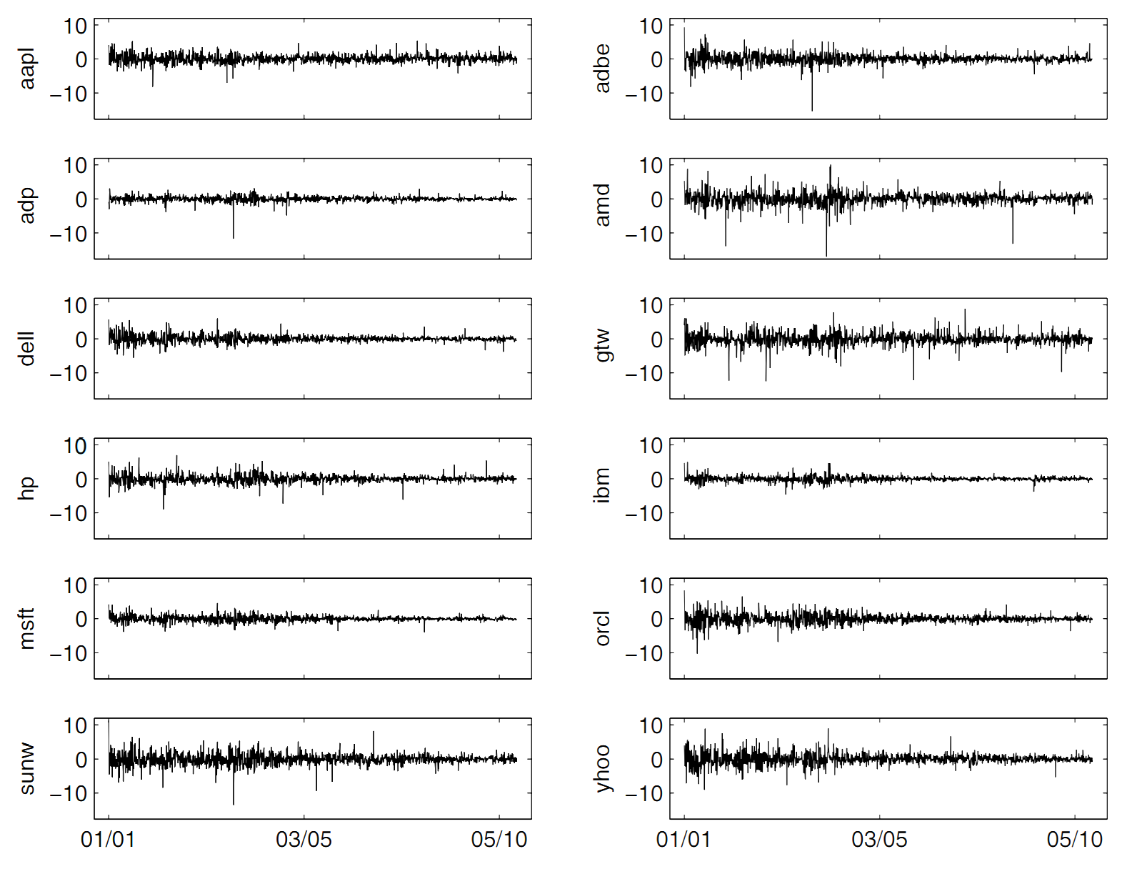
We illustrate the application of this methods in a case study that relates the daily log returns of the stock of Microsoft Corporation to those of several computer and software companies.

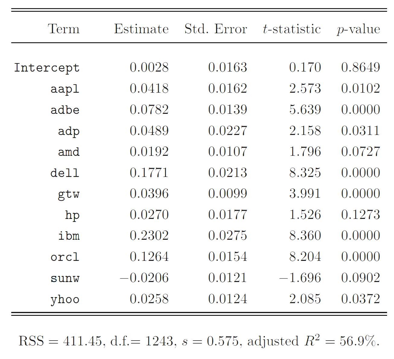
Starting with the full model, we find that the stocks hp and sunw, with relatively small partial F-statistics, are not significant at the 5% significance level. If we set the cutoff value at , which corresponds to a significance level smaller than 0.01, then hp and sunw are removed from the set of predictors after the first step. We then refit the model with the remaining predictors and repeat the backward elimination procedure with the cutoff value for the partial F-statistics. Proceeding stepwise in this way, the procedure terminates with six predictor variables: aapl, adbe, dell, gtw, ibm, orcl. The regression model can be illustrated as

Regression coefficients of the full model.

Regression coefficients of the selected regression model.

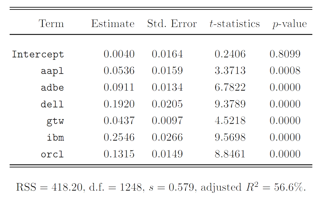
The selected model shows that, in the collection of stocks we studied, the msft daily log return is strongly influenced by those of its competitors.

Conclusion

The importance of regression analysis lies in the fact that it provides a powerful statistical method that allows a business to examine the relationship between two or more variables of interest.

References

1. Lai and Xing, Statistical Models and Methods for Financial Markets (2008)