Introduction
The aim of this project is to build a model which can make informed buy-and-sell decisions with respect to cryptocurrency trading. The model will do so by leveraging streaming news-feed data (Twitter, Bloomberg, etc.) as well as pricing data (open, close, etc.) to inform its predictions.
Configuration
Hyperparameters for neural networks.
class DictObj(object):

    def __init__(self, mp):
        import pprint
        self.map = mp
        pprint.pprint(mp)

    def __setattr__(self, name, value):
        if name == 'map':
            object.__setattr__(self, name, value)
            return
        self.map[name] = value

    def __getattr__(self, name):
        return  self.map[name]


Config = DictObj({
    "LABEL_GENERATION": "tb",
    "LAGGING": 0,
    "MAX_LENGTH": 128,
    "TRAIN_BATCH_SIZE": 128,
    "VALID_BATCH_SIZE": 128,
    "TEST_BATCH_SIZE": 128,
    "MAX_EPOCHS": 10,
    "EMBEDDING_SIZE": 300,
    "NUM_CLASSES": 2,
    "NUM_KERNELS": 128,
    "DROPOUT_RATE": 0.1
})
Load Data
The news is sourced from Bloomberg and spans the years 2014-09-23 to 2020-12-10. The row with the words “bitcoin,” “blockchain,” and “crypto” will be preserved. In terms of auto labelling, I used the Triple Barrier Method in this project because it provides the greatest results.
text_df = pd.read_csv(r"C:\Users\Yang\Desktop\Dissertation\data\processed\news\bloomberg\BloombergV2.csv")
text_df = text_df[["date", "title"]]
text_df.columns = ["date", "text"]
preprocess_func = lambda x: x.lower()
text_pipeline = TextPipeline(text_df, ["bitcoin", "blockchain", "crypto"], preprocess_func)
text_processed_df = text_pipeline.get_dataframe()

price_df = yf.download("BTC-USD", progress=False)
price_pipeline = PricePipeline(price_df, column="close", label=Config.LABEL_GENERATION)
price_processed_df = price_pipeline.get_dataframe()

text_price_pipeline = TextPricePipeline(text_processed_df, price_processed_df, lagging=Config.LAGGING)
text_price_df = text_price_pipeline.get_dataframe()
Text Preprocessing
Text processing is an automated method of evaluating and categorising unstructured text input in order to extract useful information.
def clean_text(text):
    REPLACE_BY_SPACE_RE = re.compile('[/(){}\[\]\|@,;]')
    BAD_SYMBOLS_RE = re.compile('[^0-9a-z #+_]')
    text = text.lower()
    text = REPLACE_BY_SPACE_RE.sub(' ', text)
    text = BAD_SYMBOLS_RE.sub('', text)
    text = text.strip()
    return text

text_price_df["text"] = text_price_df["text"].map(str)
text_price_df["text"] = text_price_df["text"].apply(clean_text)
Tokenisation for Train/Validation/Test Sets
Tokenisation is the process of breaking down a phrase, sentence, paragraph, or even an entire text document into smaller components like individual words or phrases.
tokenizer = AutoTokenizer.from_pretrained("bert-base-uncased")

train_df = text_price_df.loc[:"2016-12-31"]
valid_df = text_price_df.loc["2017-01-01":"2017-12-31"]
test_df = text_price_df.loc["2018-01-01":]

input_ids = tokenizer.batch_encode_plus(train_df["text"].tolist(),
                                        padding=True,
                                        truncation=True,
                                        max_length=Config.MAX_LENGTH,
                                        add_special_tokens=True,
                                        return_tensors="pt",
                                        return_token_type_ids=False,
                                        return_attention_mask=False)
X_train = input_ids["input_ids"].numpy()
y_train = train_df.label

input_ids = tokenizer.batch_encode_plus(valid_df["text"].tolist(),
                                        padding=True,
                                        truncation=True,
                                        max_length=Config.MAX_LENGTH,
                                        add_special_tokens=True,
                                        return_tensors="pt",
                                        return_token_type_ids=False,
                                        return_attention_mask=False)
X_valid = input_ids["input_ids"].numpy()
y_valid = valid_df.label

input_ids = tokenizer.batch_encode_plus(test_df["text"].tolist(),
                                        padding=True,
                                        truncation=True,
                                        max_length=Config.MAX_LENGTH,
                                        add_special_tokens=True,
                                        return_tensors="pt",
                                        return_token_type_ids=False,
                                        return_attention_mask=False)
X_test = input_ids["input_ids"].numpy()
y_test = test_df.label
Construct Dataset and Dataloader
Dataset that allow you to use pre-loaded datasets as well as your own data. Dataset stores the samples and their corresponding labels, and DataLoader wraps an iterable around the Dataset to enable easy access to the samples.
class TextDataset(torch.utils.data.Dataset):

    def __init__(self, input_ids, labels):
        self.X = input_ids
        self.y = labels

    def __len__(self):
        return len(self.y)

    def __str__(self):
        return f"<Dataset(N={len(self)})>"

    def __getitem__(self, index):
        X = self.X[index]
        y = self.y[index]
        X = torch.tensor(X, dtype=torch.long)
        y = torch.tensor(y, dtype=torch.long)
        return [X, y]

    def create_dataloader(self, batch_size, shuffle=False, drop_last=False, num_workers=0):
        return torch.utils.data.DataLoader(
            dataset=self,
            batch_size=batch_size,
            shuffle=shuffle,
            drop_last=drop_last,
            pin_memory=True,
            num_workers=num_workers)

train_dataset = TextDataset(X_train, y_train)
valid_dataset = TextDataset(X_valid, y_valid)
test_dataset = TextDataset(X_test, y_test)

train_dataloader = train_dataset.create_dataloader(batch_size=Config.TRAIN_BATCH_SIZE, shuffle=True)
valid_dataloader = valid_dataset.create_dataloader(batch_size=Config.VALID_BATCH_SIZE)
test_dataloader = test_dataset.create_dataloader(batch_size=Config.TEST_BATCH_SIZE)
Modelling
Building representations of things in the ‘real world’ and allowing concepts to be probed is what modelling is all about.
Pytorch Lightning Module
Pytorch Lightning structures PyTorch code so it can abstract the details of training.
class LightningMultiClassModule(pl.LightningModule):
    """
    Multi-class Classification Engine
    """

    learning_rate = 1e-3

    def __init__(self):
        super().__init__()
        self.train_losses = []
        self.valid_losses = []
        self.train_accuracies = []
        self.valid_accuracies = []

    def forward(self, inputs):
        raise NotImplementedError

    def configure_optimizers(self):
        optimizer = torch.optim.Adam(self.parameters(), lr=self.learning_rate)
        return optimizer

    def training_step(self, batch, batch_idx):
        batch, y = batch
        y_hat = self(batch)
        labels_hat = torch.argmax(y_hat, dim=1)
        n_correct_pred = torch.sum(y == labels_hat).item()
        loss = F.cross_entropy(y_hat, y.long())
        self.log("train_loss", loss, on_step=True, on_epoch=True, logger=False)
        return {'loss': loss, "n_correct_pred": n_correct_pred, "n_pred": len(y)}

    def training_epoch_end(self, outputs):
        avg_loss = torch.stack([x['loss'] for x in outputs]).mean()
        train_acc = sum([x['n_correct_pred'] for x in outputs]) / sum(x['n_pred'] for x in outputs)
        self.train_losses.append(avg_loss.detach().cpu().item())
        self.train_accuracies.append(train_acc)

    def validation_step(self, batch, batch_idx):
        batch, y = batch
        y_hat = self(batch)
        loss = F.cross_entropy(y_hat, y.long())
        labels_hat = torch.argmax(y_hat, dim=1)
        n_correct_pred = torch.sum(y == labels_hat).item()
        self.log("valid_loss", loss, on_step=True, on_epoch=True, logger=False)
        return {'val_loss': loss, "n_correct_pred": n_correct_pred, "n_pred": len(y)}

    def validation_epoch_end(self, outputs):
        avg_loss = torch.stack([x['val_loss'] for x in outputs]).mean()
        val_acc = sum([x['n_correct_pred'] for x in outputs]) / sum(x['n_pred'] for x in outputs)
        self.valid_losses.append(avg_loss.detach().cpu().item())
        self.valid_accuracies.append(val_acc)

    def test_step(self, batch, batch_idx):
        batch, y = batch
        y_hat = self(batch)
        loss = F.cross_entropy(y_hat, y.long())
        labels_hat = torch.argmax(y_hat, dim=1)
        n_correct_pred = torch.sum(y == labels_hat).item()

        return {'test_loss': loss, "n_correct_pred": n_correct_pred, "n_pred": len(y)}

    def test_epoch_end(self, outputs):
        avg_loss = torch.stack([x['test_loss'] for x in outputs]).mean()
        test_acc = sum([x['n_correct_pred'] for x in outputs]) / sum(x['n_pred'] for x in outputs)

    def predict_proba(self, test_dataloader):
        """Prediction Step"""
        # Set model to eval mode
        self.eval()
        y_probs = []

        # Iterate over val batches
        with torch.no_grad():
            for i, batch in enumerate(tqdm(test_dataloader)):
                x, y = batch
                x, y = x.to(self.device), y.to(self.device)
                # Forward pass with inputs
                y_prob = self(x)
                # Store outputs
                y_probs.extend(y_prob.cpu())

        return softmax(np.vstack(y_probs), axis=1)
TextCNN
The convolutional neural network for text, or TextCNN, is a helpful deep learning technique for tasks including sentiment analysis and question classification.
class TextCNN(LightningMultiClassModule):
    """
    https://finisky.github.io/2020/07/03/textcnnmvp/
    """
    def __init__(self, embed_num, embed_dim, class_num, kernel_num=100, kernel_sizes=[3, 4, 5], dropout=0.5):
        super(TextCNN, self).__init__()

        Ci = 1
        Co = kernel_num

        self.embed = nn.Embedding(embed_num, embed_dim)
        self.convs = nn.ModuleList([nn.Conv2d(Ci, Co, (f, embed_dim), padding=(2, 0)) for f in kernel_sizes])

        self.dropout = nn.Dropout(dropout)
        self.fc = nn.Linear(Co * len(kernel_sizes), class_num)

    def forward(self, x):
        x = self.embed(x)                                         # (N, token_num, embed_dim)
        x = x.unsqueeze(1)                                        # (N, Ci, token_num, embed_dim)
        x = [F.relu(conv(x)).squeeze(3) for conv in self.convs]   # [(N, Co, token_num) * len(kernel_sizes)]
        x = [F.max_pool1d(i, i.size(2)).squeeze(2) for i in x]    # [(N, Co) * len(kernel_sizes)]
        x = torch.cat(x, 1)                                       # (N, Co * len(kernel_sizes))
        x = self.dropout(x)                                       # (N, Co * len(kernel_sizes))
        logit = self.fc(x)                                        # (N, class_num)
        return logit

    def configure_optimizers(self):
        optimiser = torch.optim.Adam(self.parameters(), lr=self.learning_rate)
        # scheduler = torch.optim.lr_scheduler.StepLR(optimizer, step_size=1, gamma=0.1)
        # return [optimizer], [scheduler]
        return optimiser

def init_weights(m):
    if type(m) == nn.Linear:
        torch.nn.init.xavier_uniform(m.weight)
        m.bias.data.fill_(0.01)
Start Training Process
The process of training an ML model entails sending training data to an ML algorithm (that is, the learning algorithm).
textcnn = TextCNN(embed_num=len(tokenizer.vocab),
                  embed_dim=Config.EMBEDDING_SIZE,
                  class_num=Config.NUM_CLASSES,
                  kernel_num=Config.NUM_KERNELS,
                  kernel_sizes=[3, 4, 5],
                  dropout=Config.DROPOUT_RATE)
textcnn.learning_rate = 3e-5
textcnn.apply(init_weights)
trainer = pl.Trainer(gpus=1, precision=16, fast_dev_run=False, max_epochs=20, num_sanity_val_steps=0)
trainer.fit(textcnn, train_dataloader, valid_dataloader)
Performance
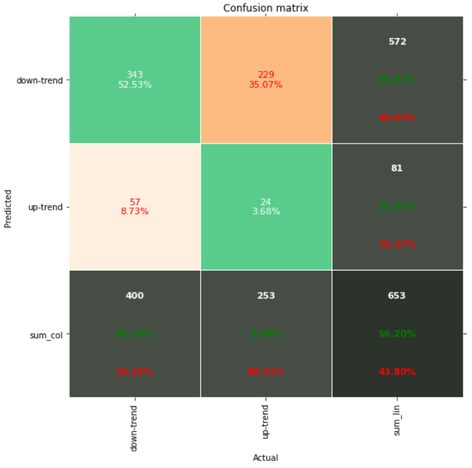
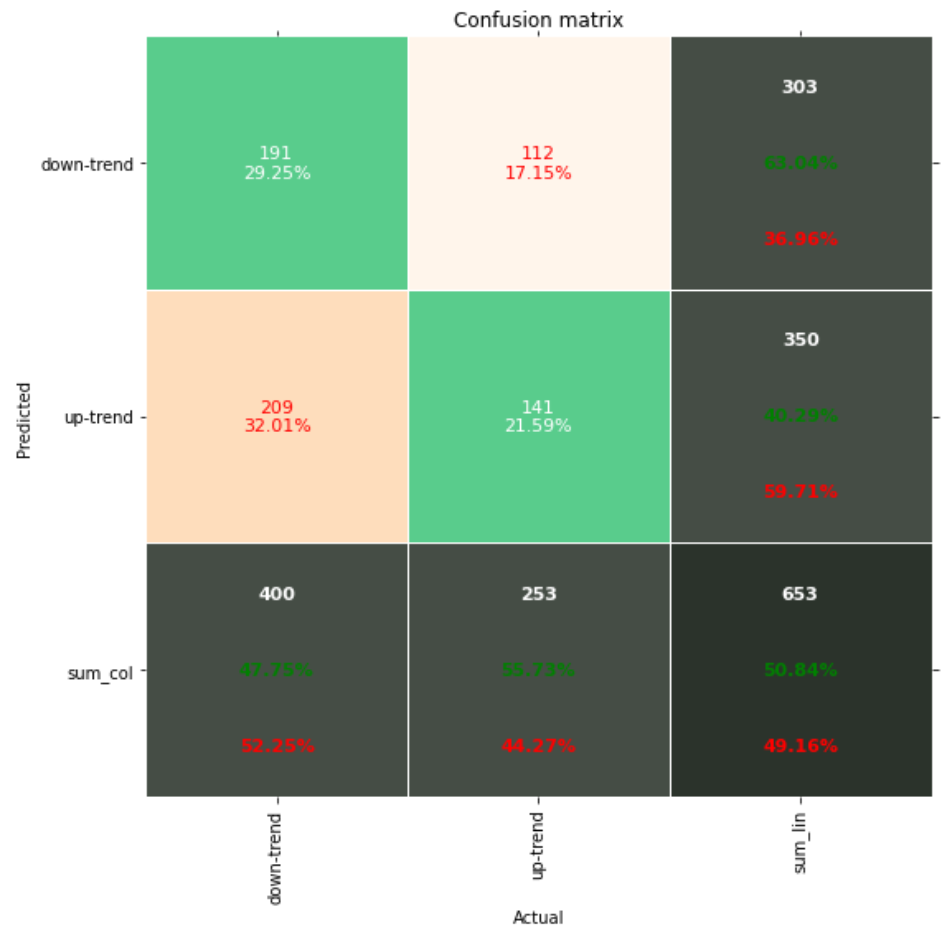
After training 20 epochs, we can get f1 score of 48.7999% and accuracy of 56.2021%.
test_probs = textcnn.predict_proba(test_dataloader)
test_preds = np.argmax(test_probs, axis=1)
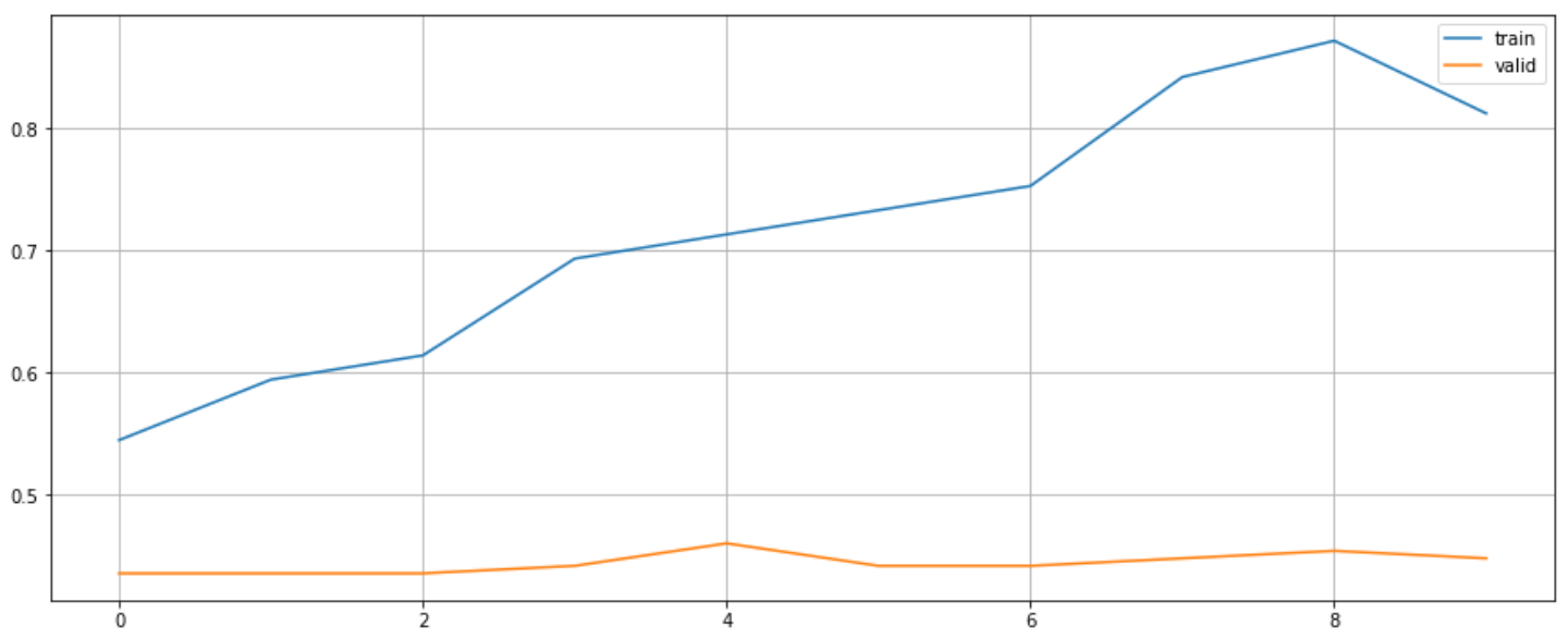
metrics.f1_score(y_test, test_preds, average="weighted"), metrics.accuracy_score(y_test, test_preds)Accuracy curve is as follow.
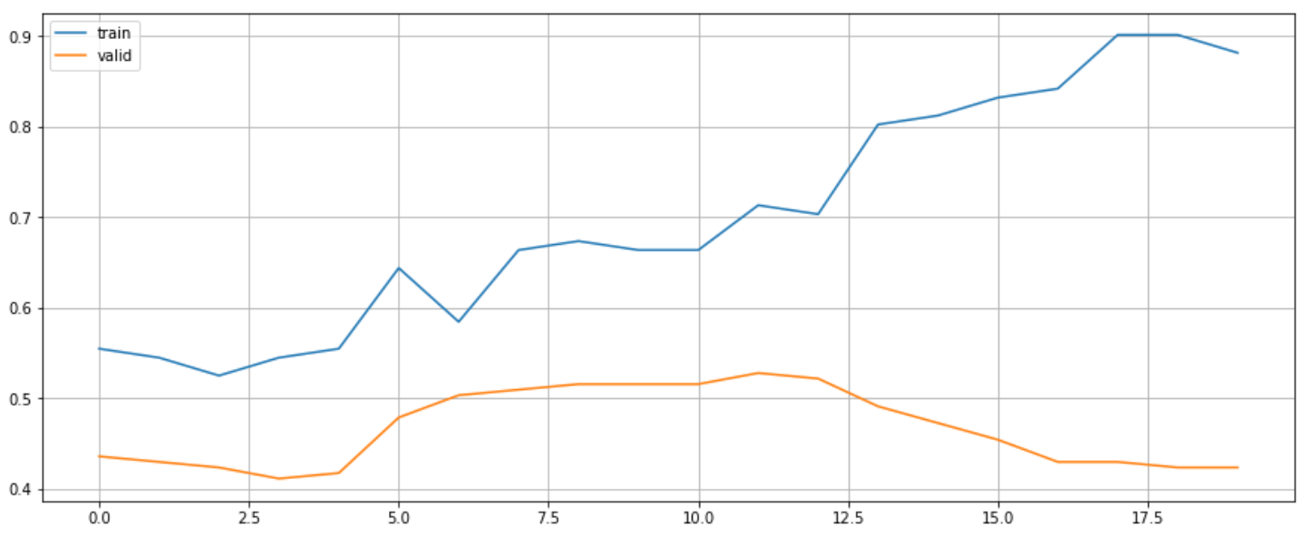
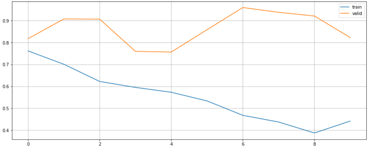
Loss curve is as follow.
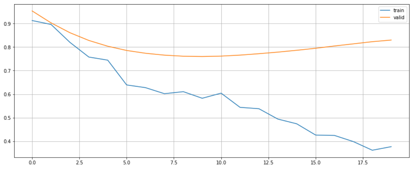
Confusion matrix is as follow.
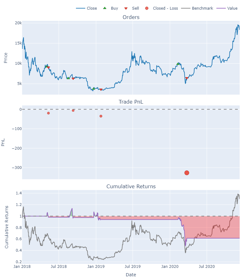
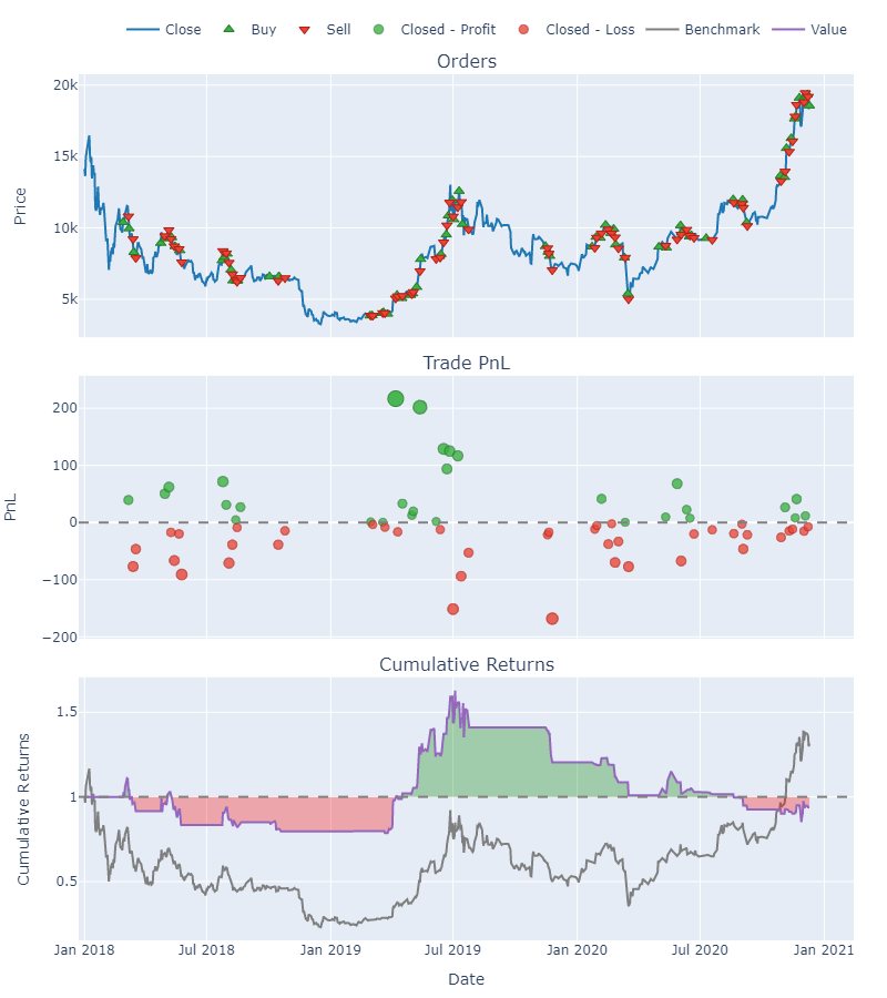
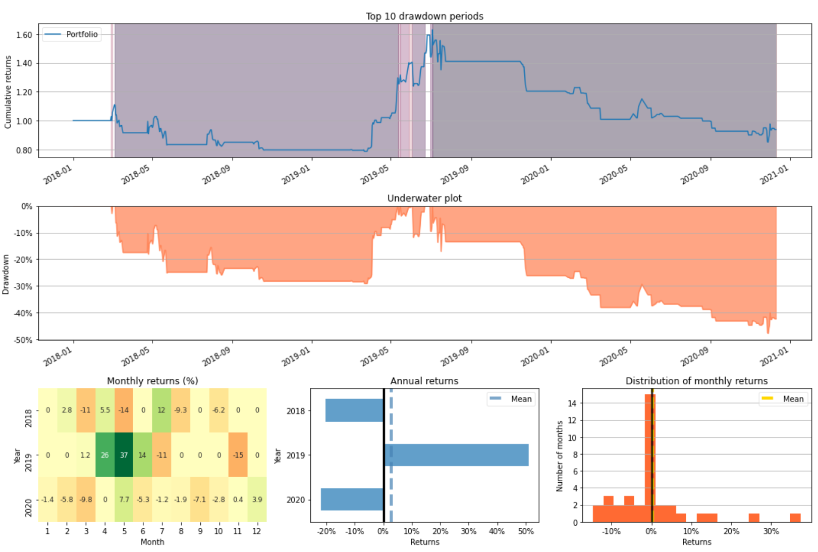
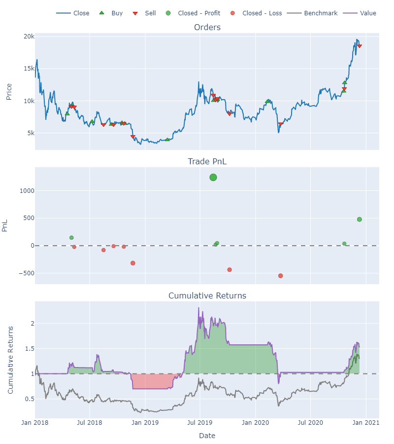
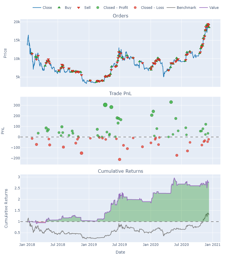
Backtest
Backtesting is a way for determining how well a strategy or model would have performed in the absence of the strategy or model. Backtesting is a method of determining the viability of a trading strategy by examining how it would perform in the real world using previous data. If backtesting proves to be effective, traders and analysts may be more willing to use it in the future.
trends = np.argmax(test_probs, axis=1)
entries, exits = trend_to_signal(pd.Series(trends))
price_test = text_price_df.iloc[-X_test.shape[0]:]
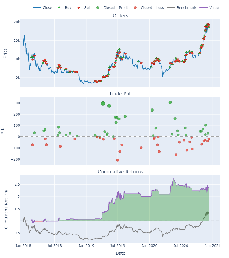
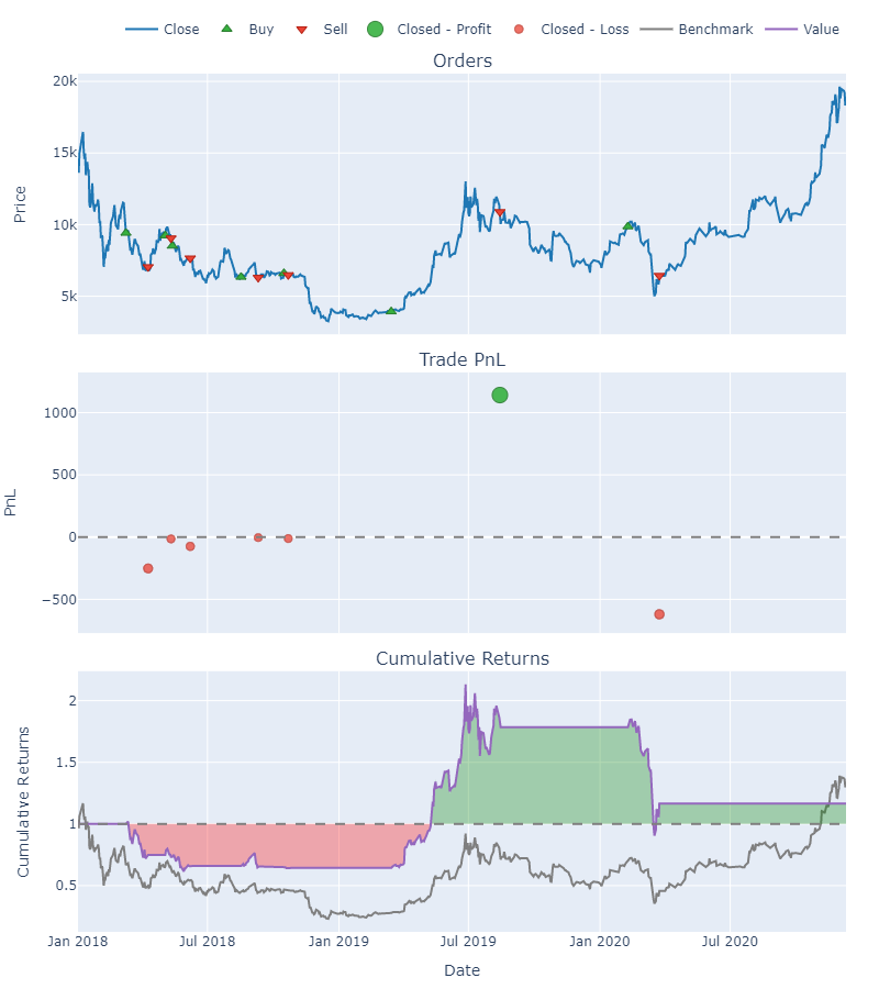
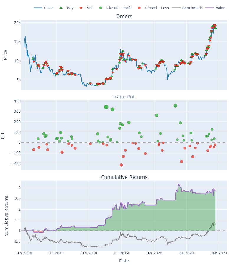
mlbp_textcnn = MachineLearningBacktestPortfolio(price_test.open,
entries,
exits,
show=True)
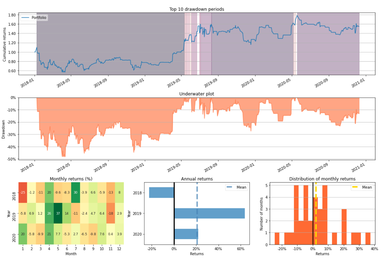
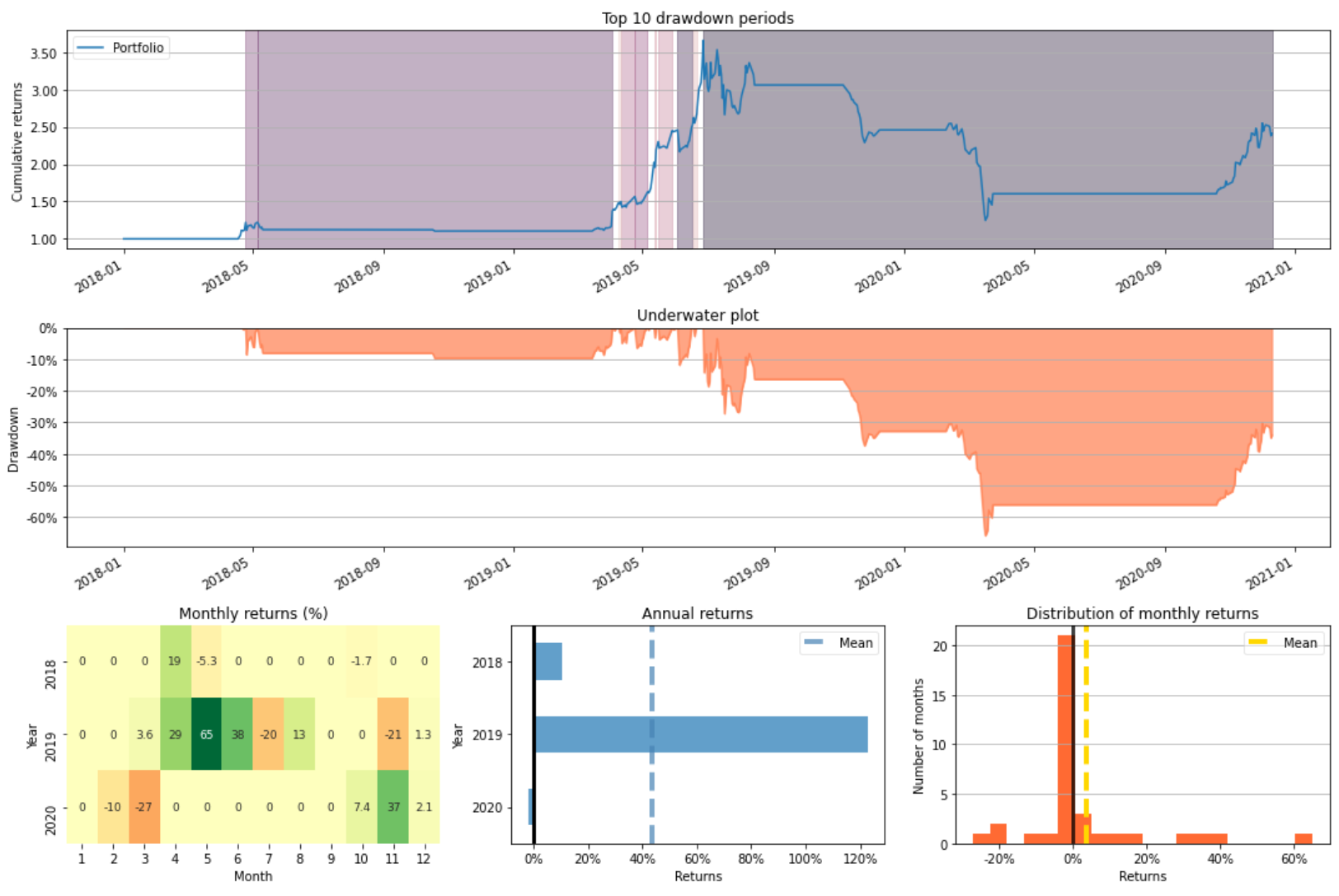
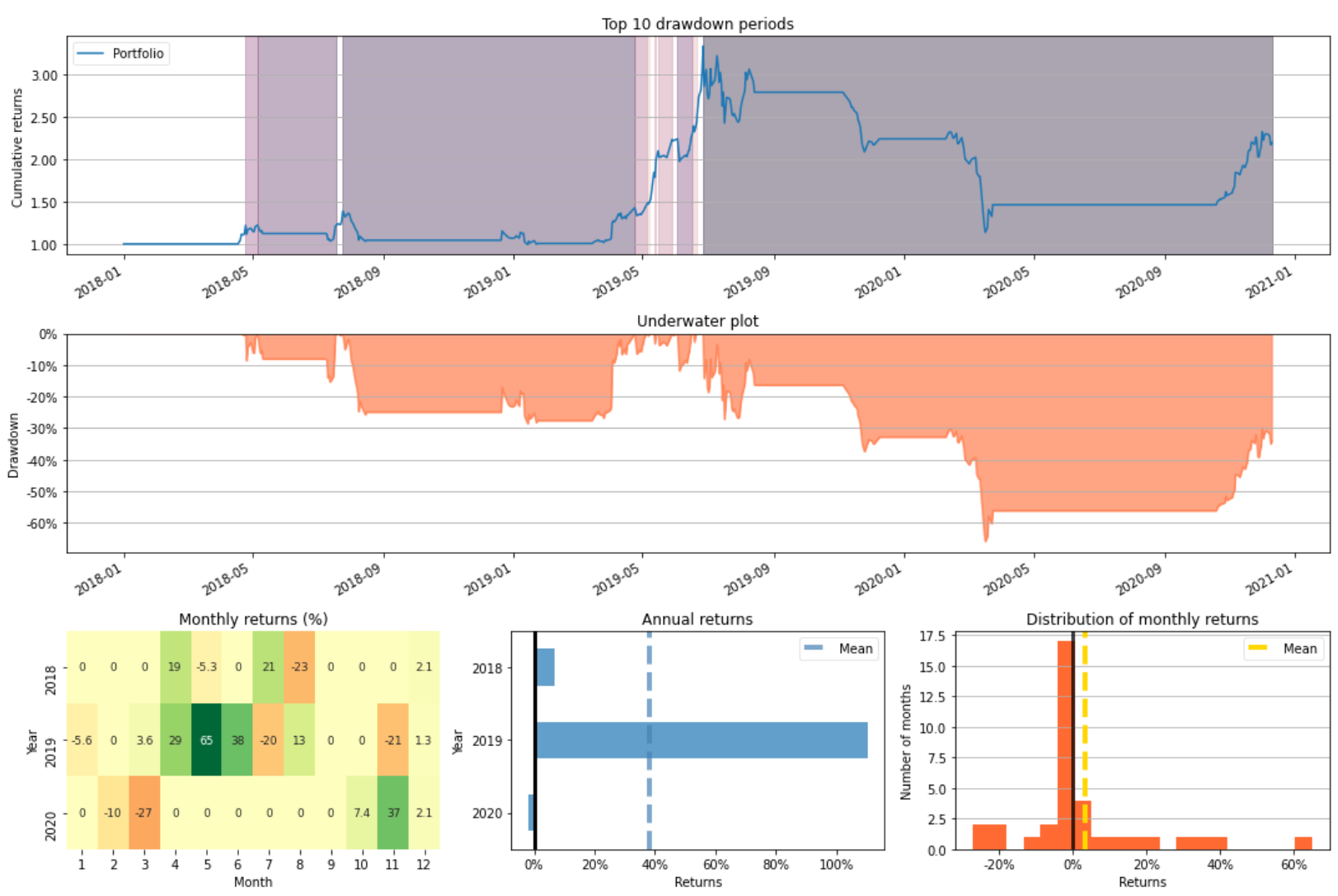
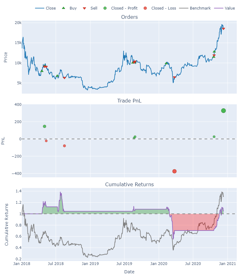
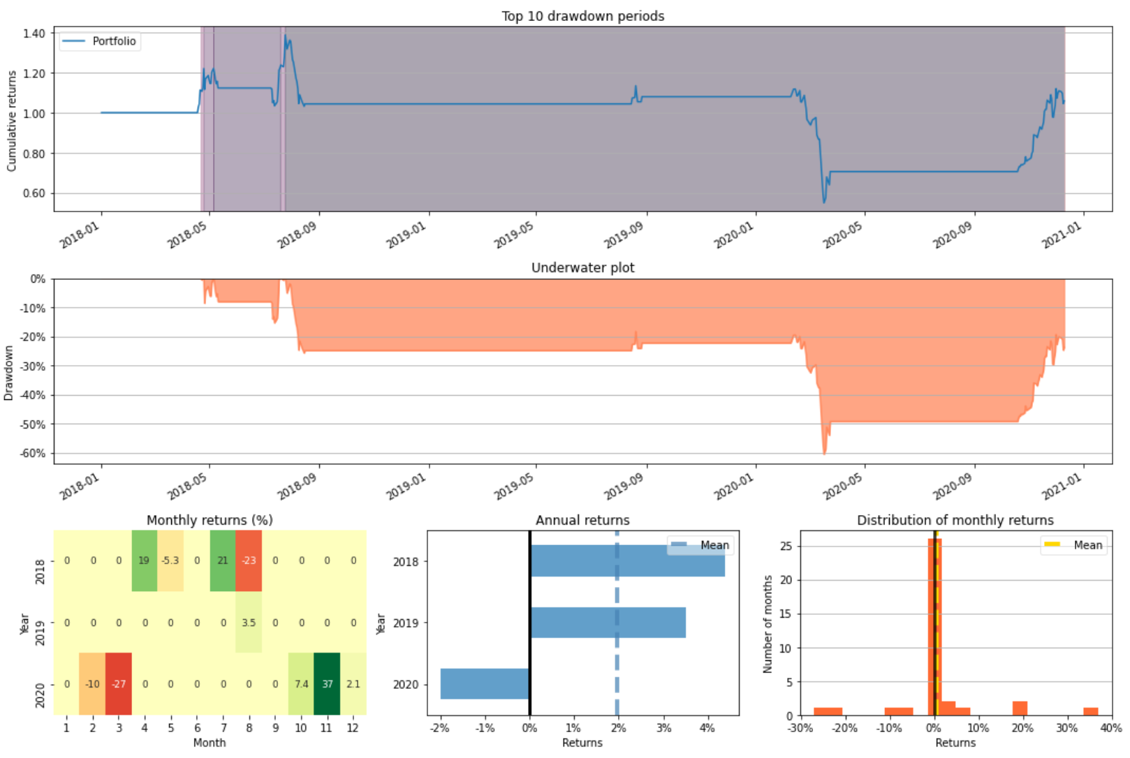
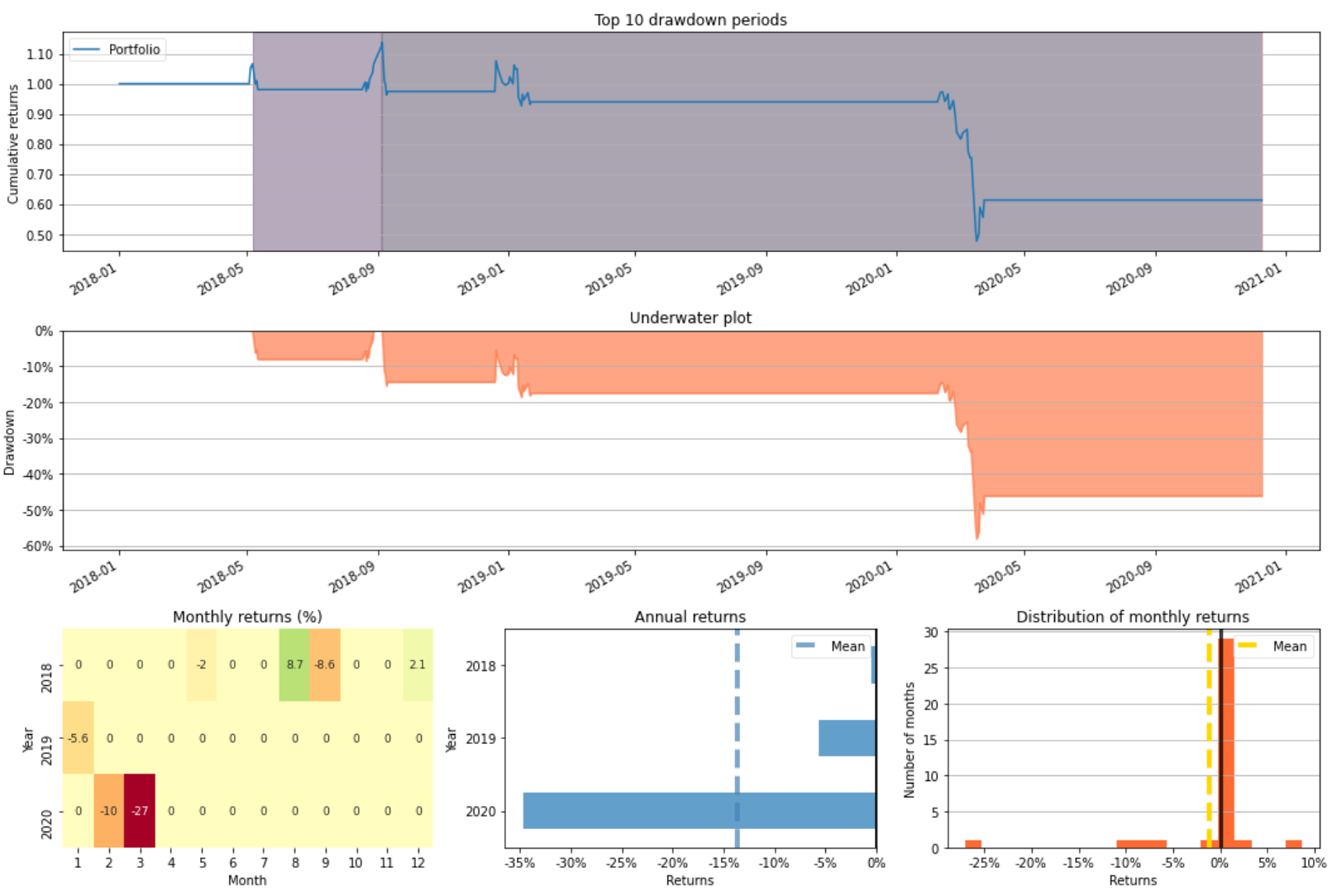
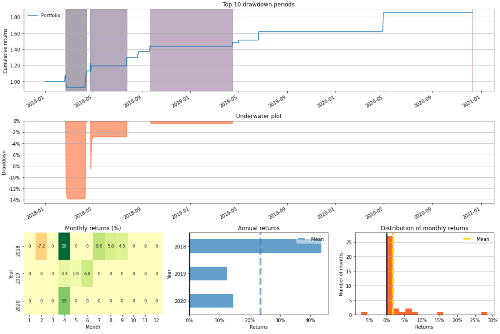
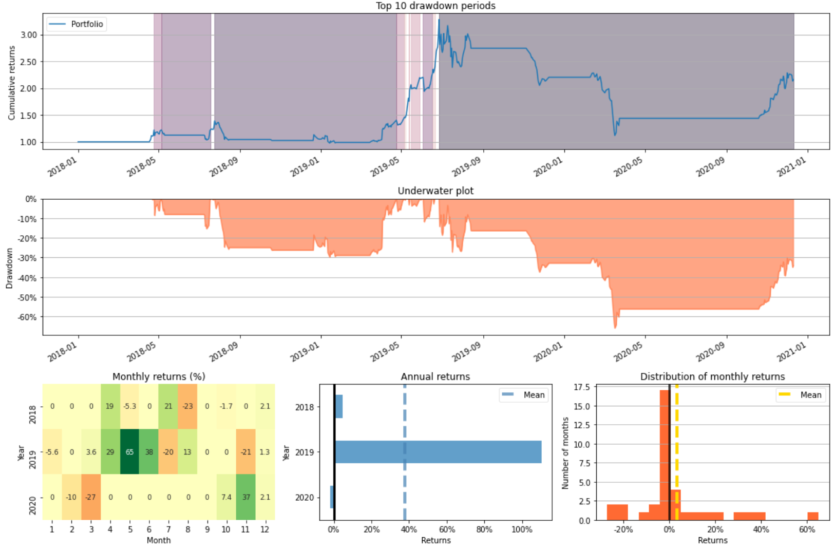
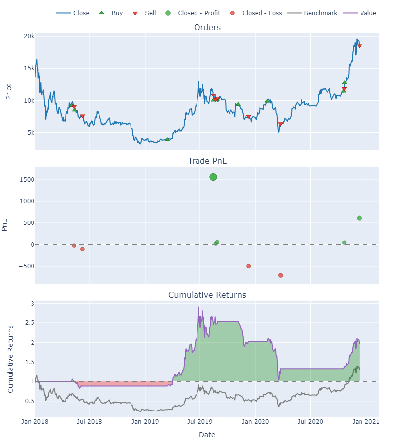
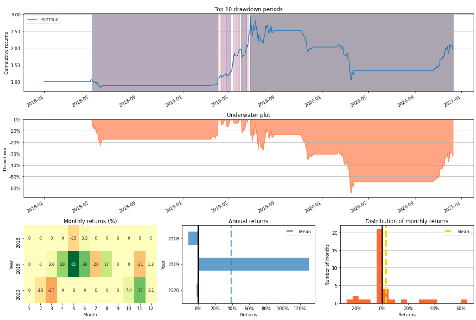
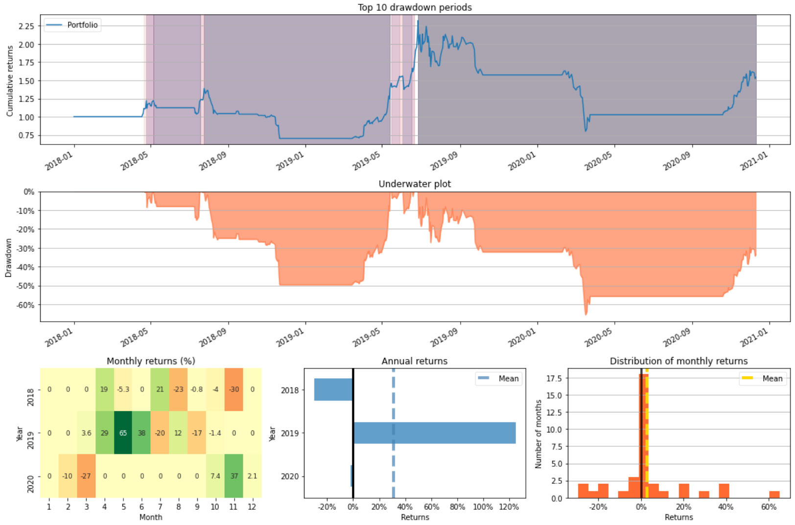
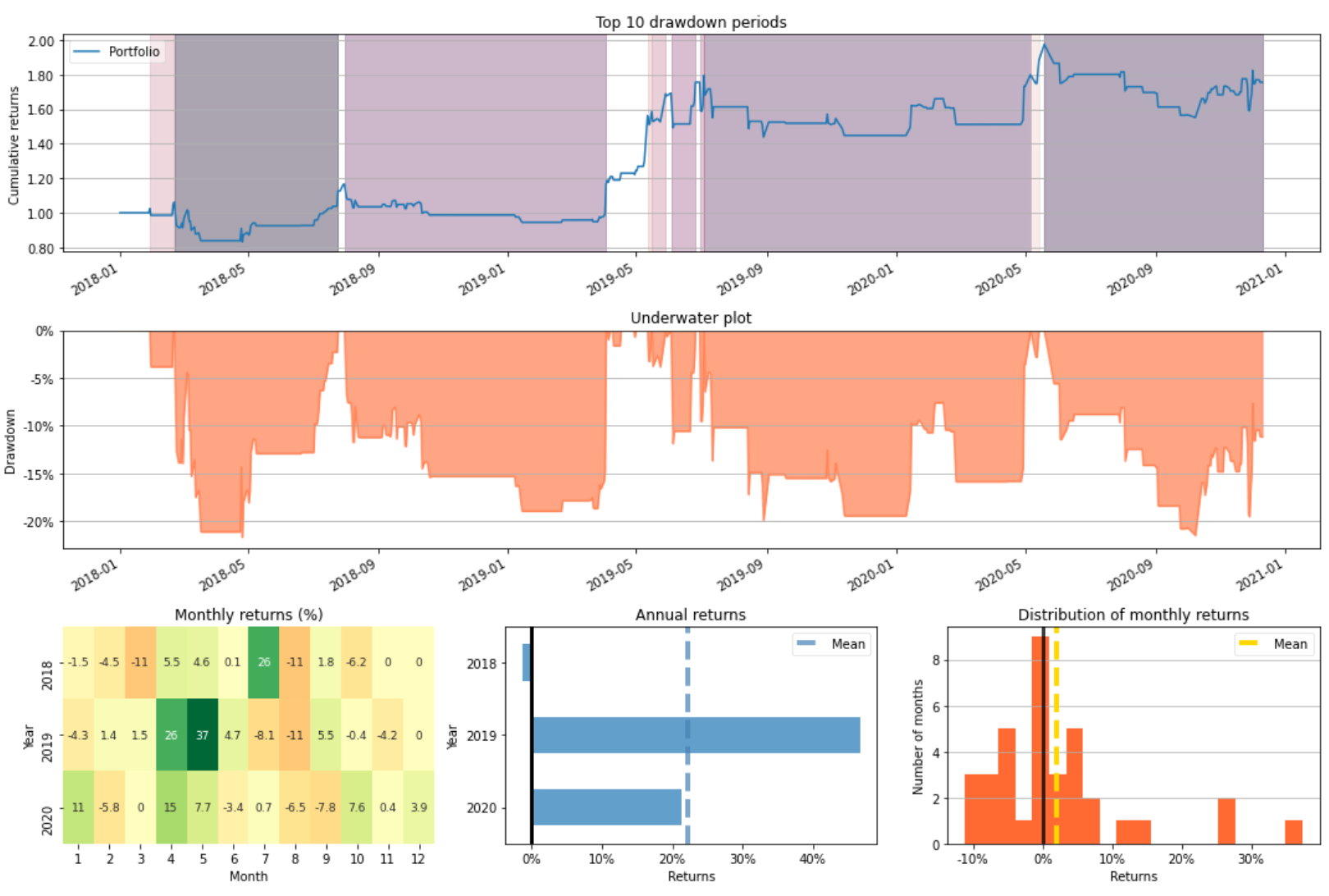
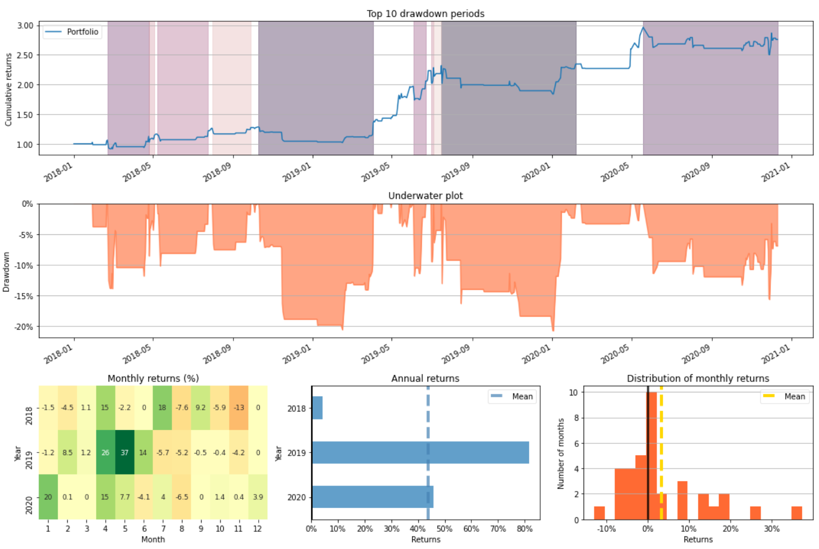
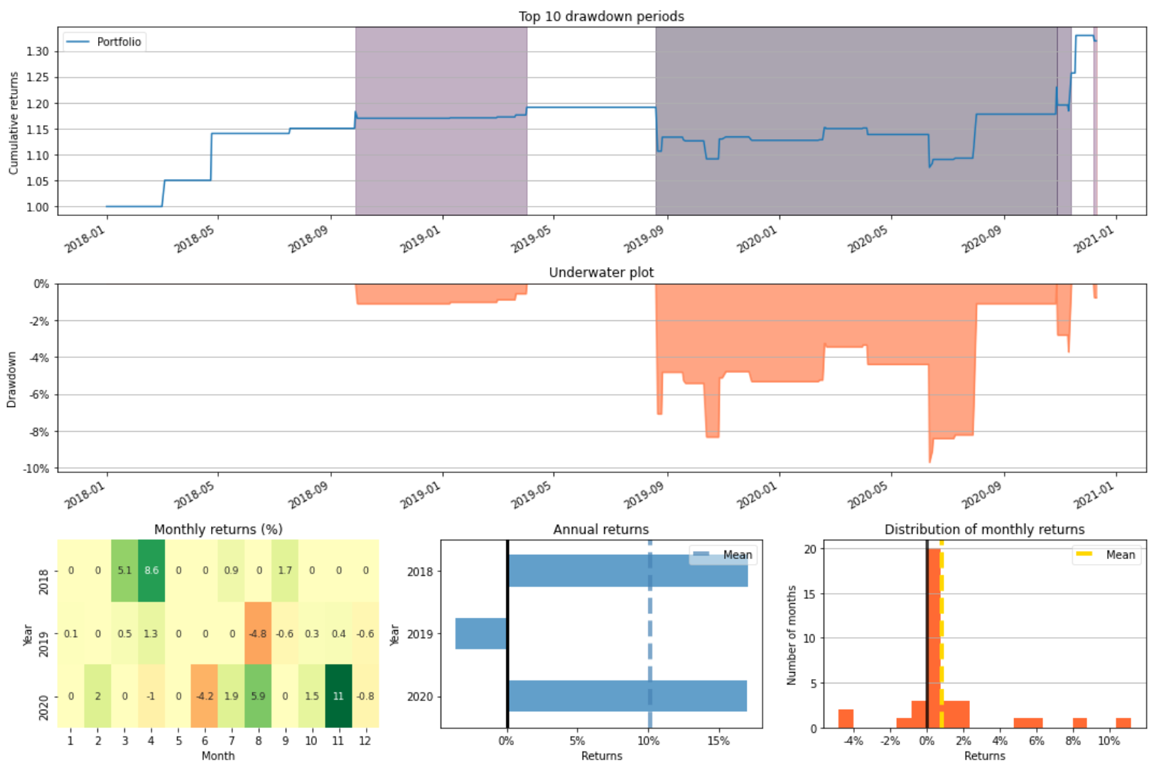
mlbp_textcnn.plot_risk(figsize=(15, 10))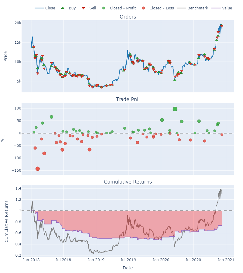
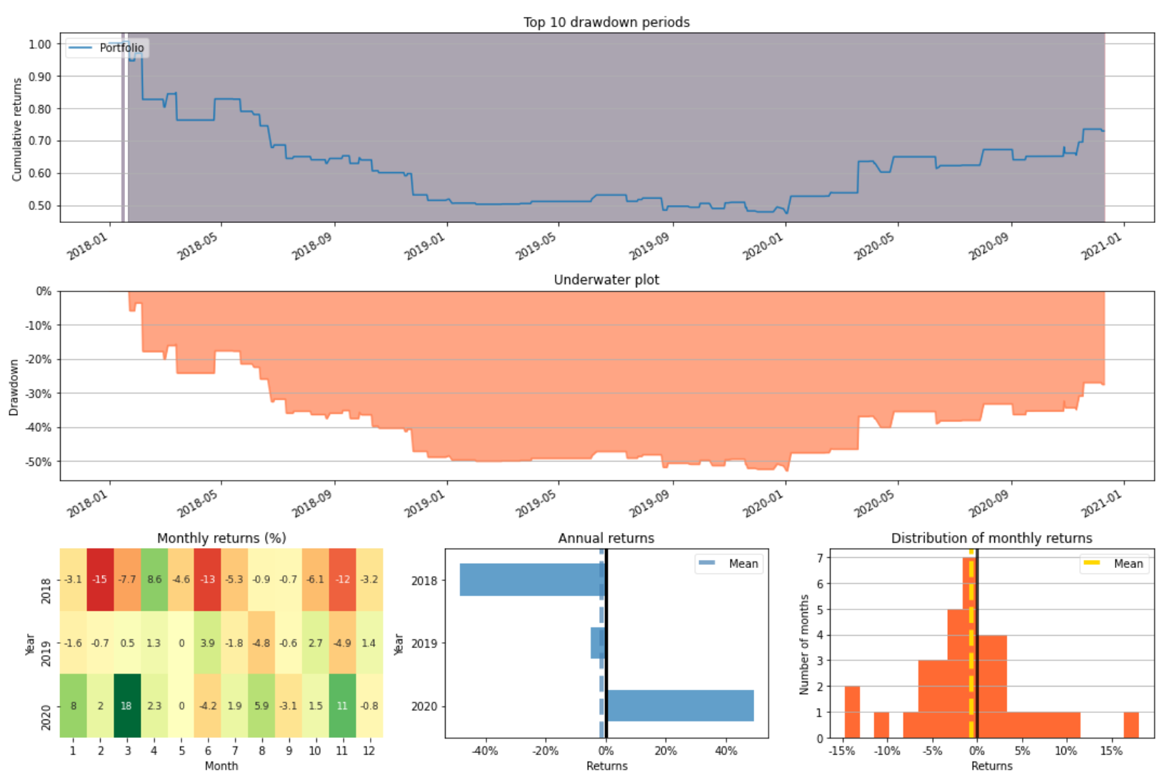
Start                           2018-01-01 00:00:00
End                             2020-12-10 00:00:00
Duration                          653 days 00:00:00
Init. Cash                                   1000.0
Total Profit                            -271.728922
Total Return [%]                         -27.172892
Benchmark Return [%]                      31.469924
Position Coverage [%]                     12.404288
Max. Drawdown [%]                         52.866542
Avg. Drawdown [%]                         26.433271
Max. Drawdown Duration            636 days 00:00:00
Avg. Drawdown Duration            319 days 00:00:00
Num. Trades                                      70
Win Rate [%]                              51.428571
Best Trade [%]                            18.039317
Worst Trade [%]                          -14.736523
Avg. Trade [%]                            -0.335031
Max. Trade Duration                 3 days 00:00:00
Avg. Trade Duration       1 days 03:46:17.142857142
Expectancy                                -3.881842
SQN                                        -0.96268
Gross Exposure                             0.124043
Sharpe Ratio                              -0.418759
Sortino Ratio                             -0.581125
Calmar Ratio                              -0.307222
BERT
Google created a Transformer-based machine learning methodology for natural language processing pre-training called Bidirectional Encoder Representations from Transformers. Jacob Devlin and his Google colleagues designed and published BERT in 2018.
from transformers import BertModel, AdamW

class BERTBaseUncased(LightningMultiClassModule):

    def __init__(self, num_classes, learning_rate=3e-5):
        super(BERTBaseUncased, self).__init__()
        self.learning_rate = learning_rate
        self.bert = BertModel.from_pretrained("bert-base-uncased")
        self.dropout = nn.Dropout(0.3)
        self.bn = nn.BatchNorm1d(768)
        self.classifier = nn.Linear(768, num_classes)

    def forward(self, x):
        outputs = self.bert(x)
        b_o = self.dropout(outputs.pooler_output)
        logits = self.classifier(self.bn(b_o))
        return logits

    def freeze_bert_encoder(self):
        for param in self.bert.parameters():
            param.requires_grad = False

    def unfreeze_bert_encoder(self):
        for param in self.bert.parameters():
            param.requires_grad = True

    def configure_optimizers(self):
        optimizer = AdamW(self.parameters(), lr=self.learning_rate)
        return optimizer
Start Training Process
bert = BERTBaseUncased(num_classes=Config.NUM_CLASSES)
bert.unfreeze_bert_encoder()
trainer = pl.Trainer(gpus=1,
                     precision=16,
                     fast_dev_run=False,
                     max_epochs=10,
                     num_sanity_val_steps=0,
                     deterministic=True)
trainer.fit(bert, train_dataloader, valid_dataloader)
Performance
After training 20 epochs, we can get f1 score of 51.4047% and accuracy of 50.8423%.
test_probs = bert.predict_proba(test_dataloader)
test_preds = np.argmax(test_probs, axis=1)
metrics.f1_score(y_test, test_preds, average="weighted"), metrics.accuracy_score(y_test, test_preds)
Accuracy curve is as follow.
Loss curve is as follow.
Confusion matrix is as follow.
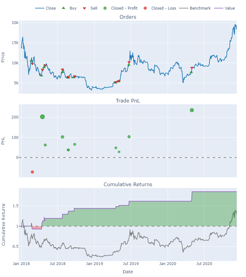
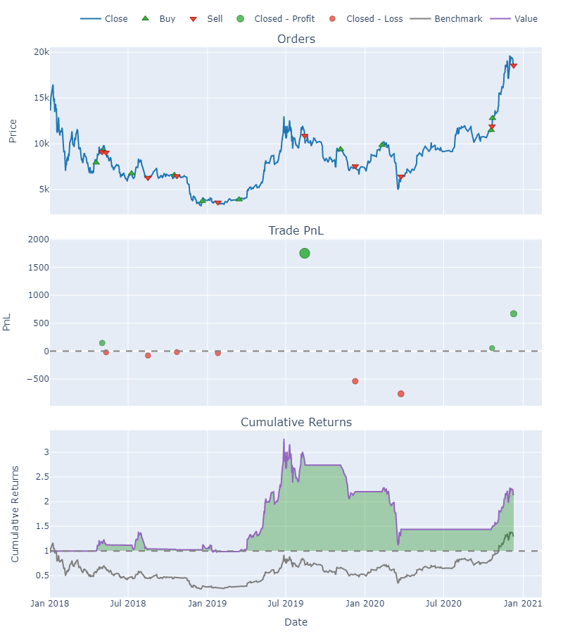
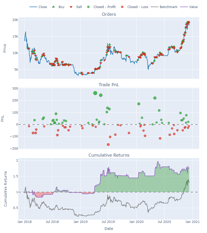
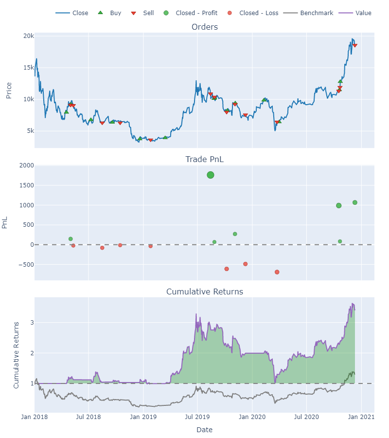
Backtest
trends = np.argmax(test_probs, axis=1)
entries, exits = trend_to_signal(pd.Series(trends))
price_test = text_price_df.iloc[-X_test.shape[0]:]
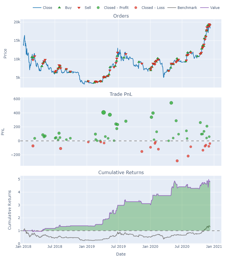
mlbp_bert = MachineLearningBacktestPortfolio(price_test.open,
entries,
exits,
show=True)
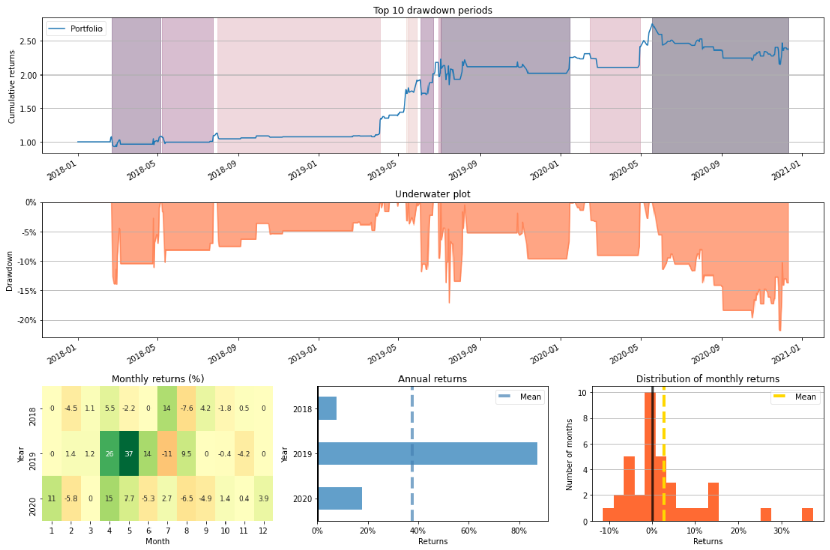
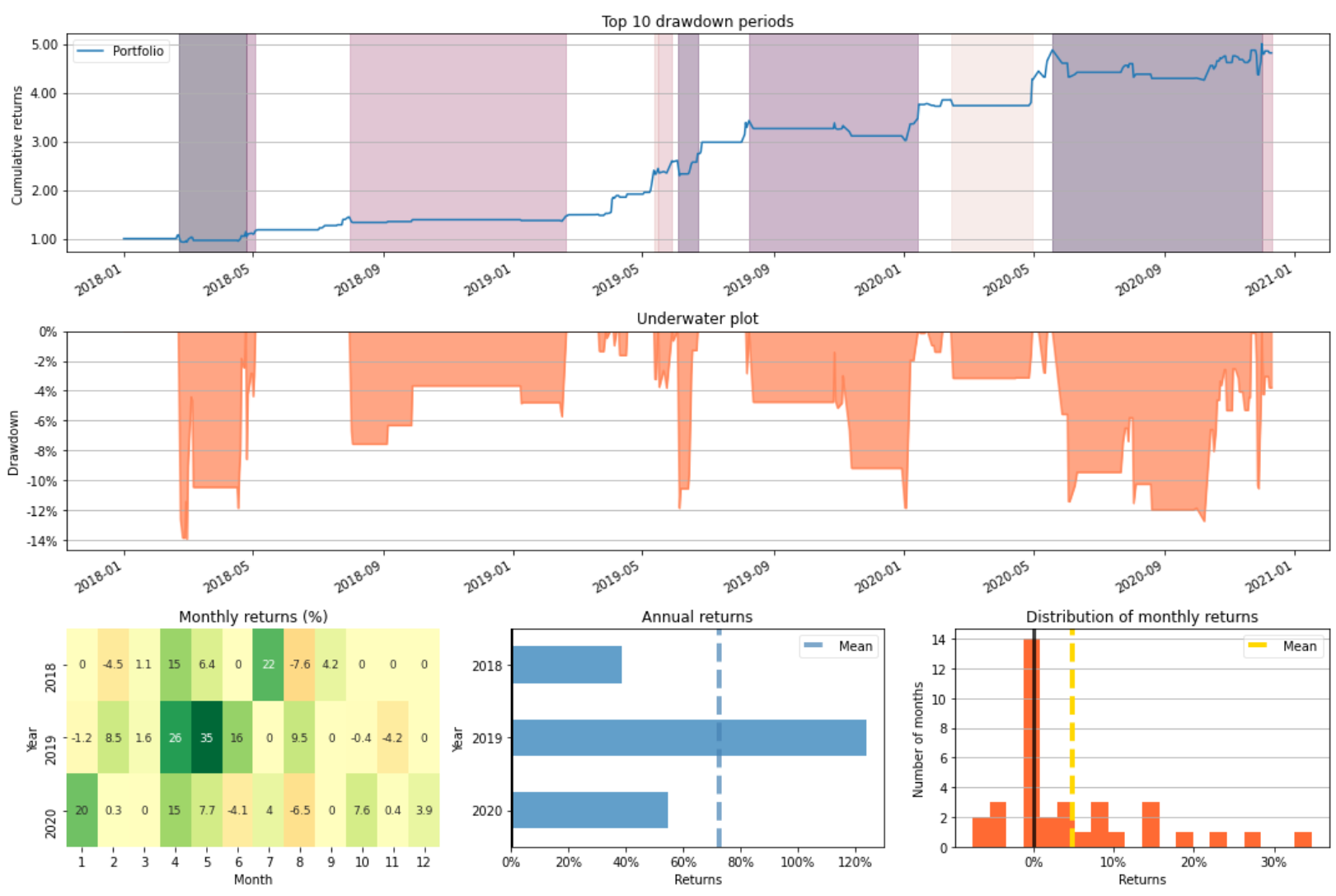
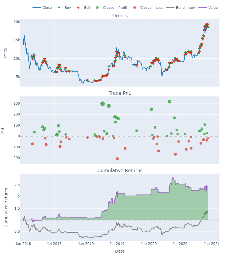
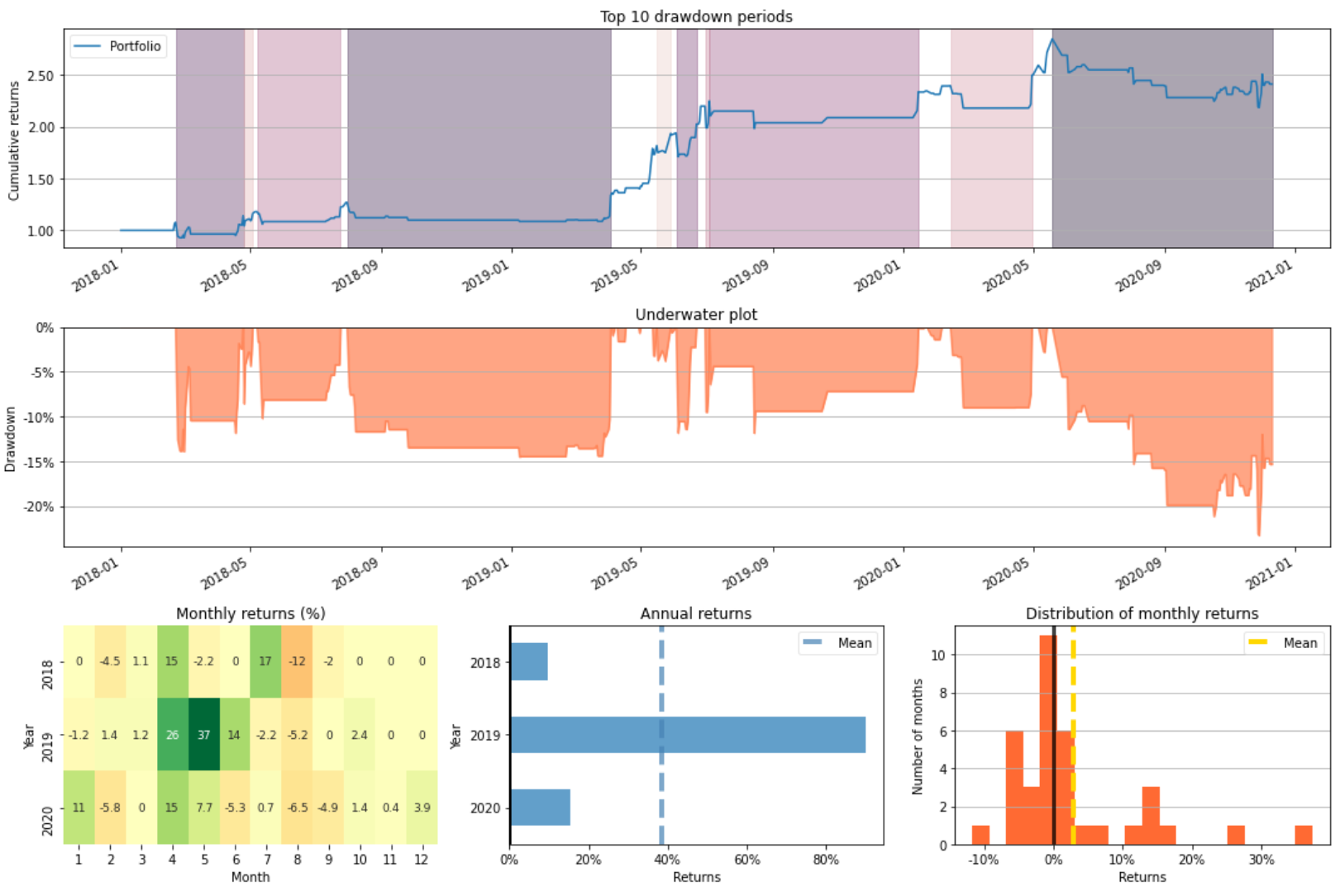
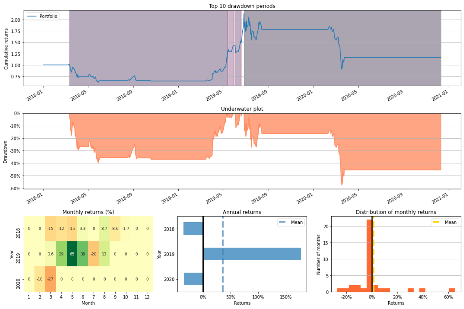
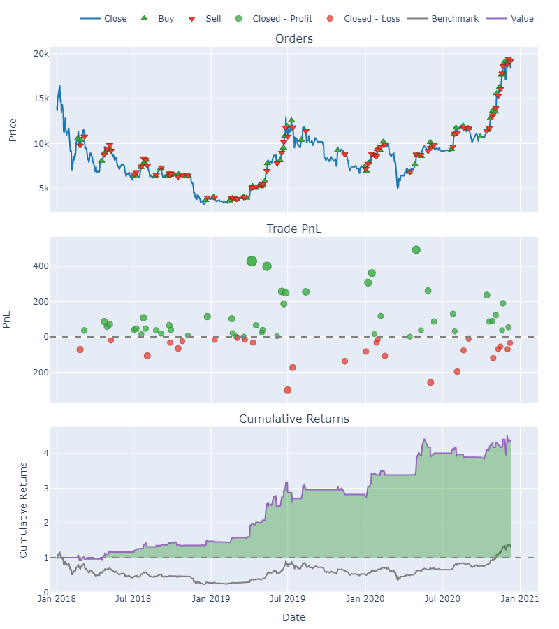
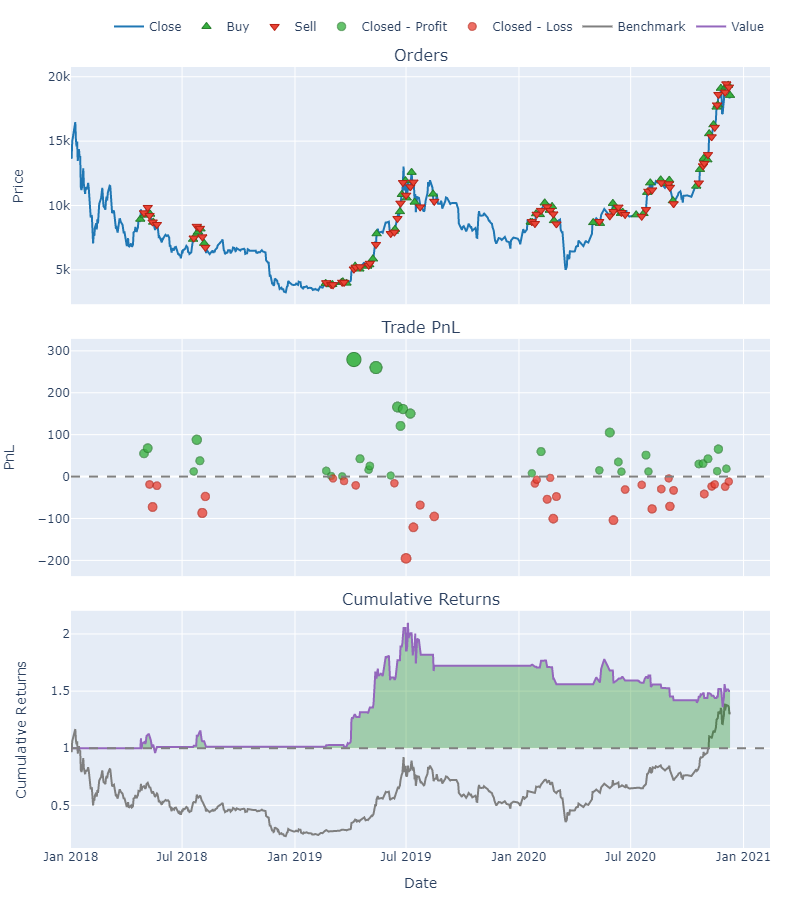
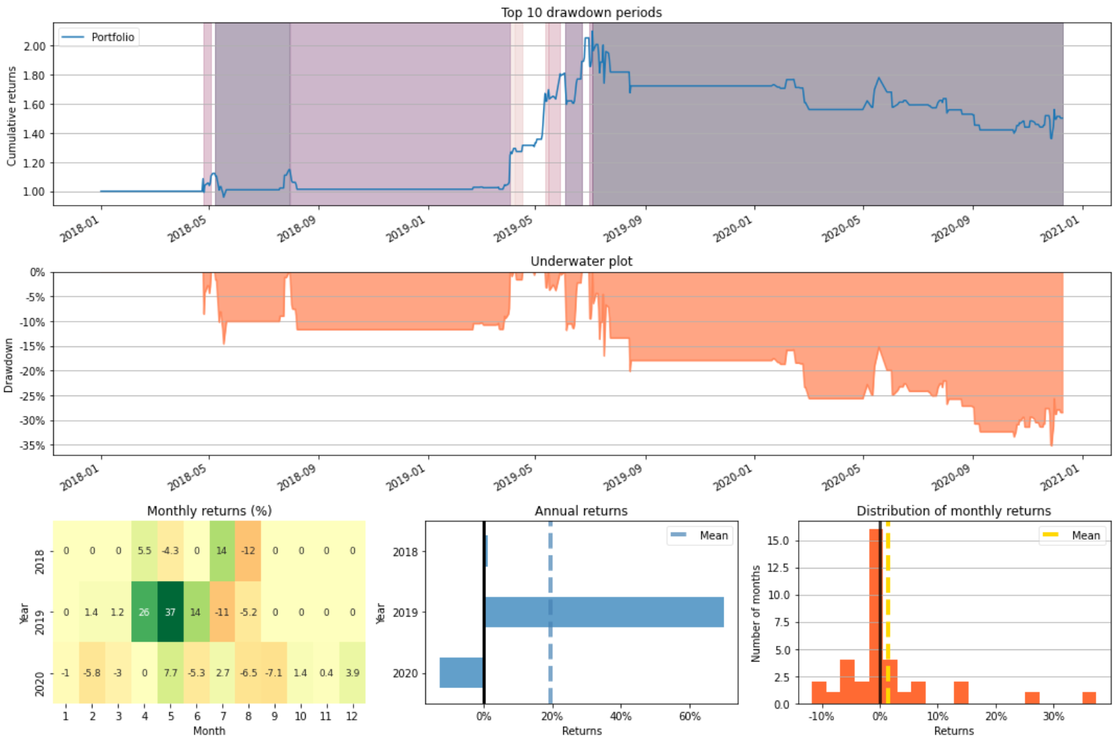
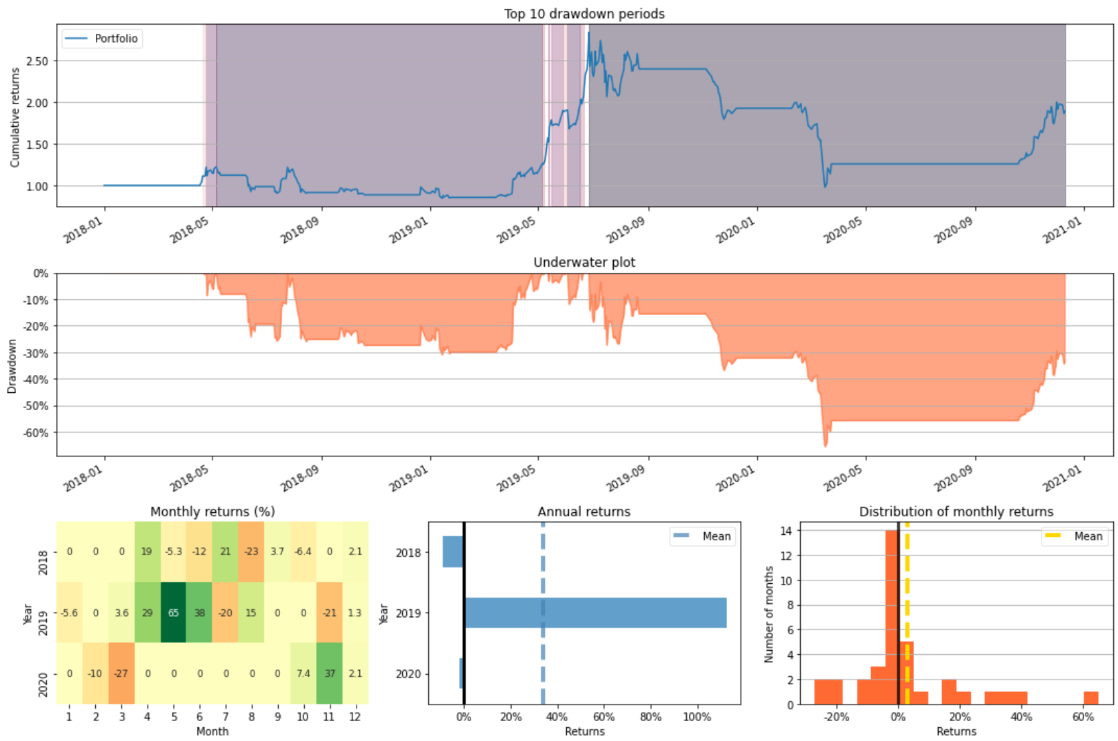
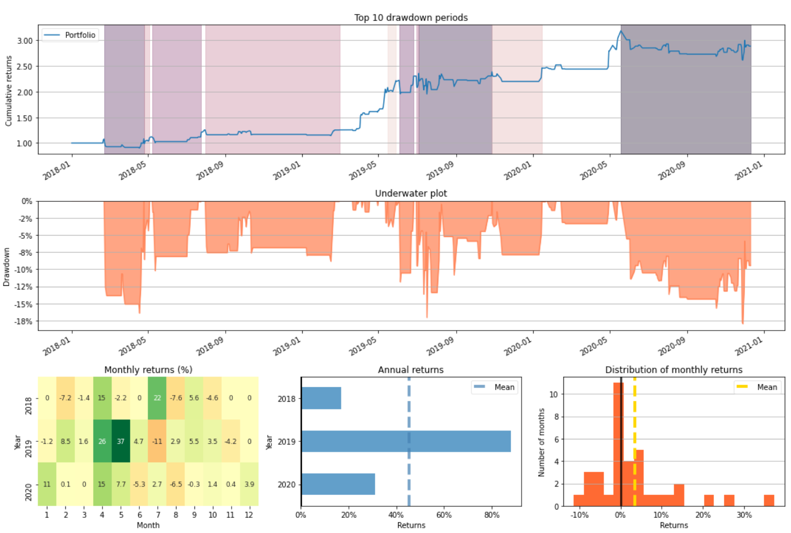
mlbp_bert.plot_risk(figsize=(15, 10))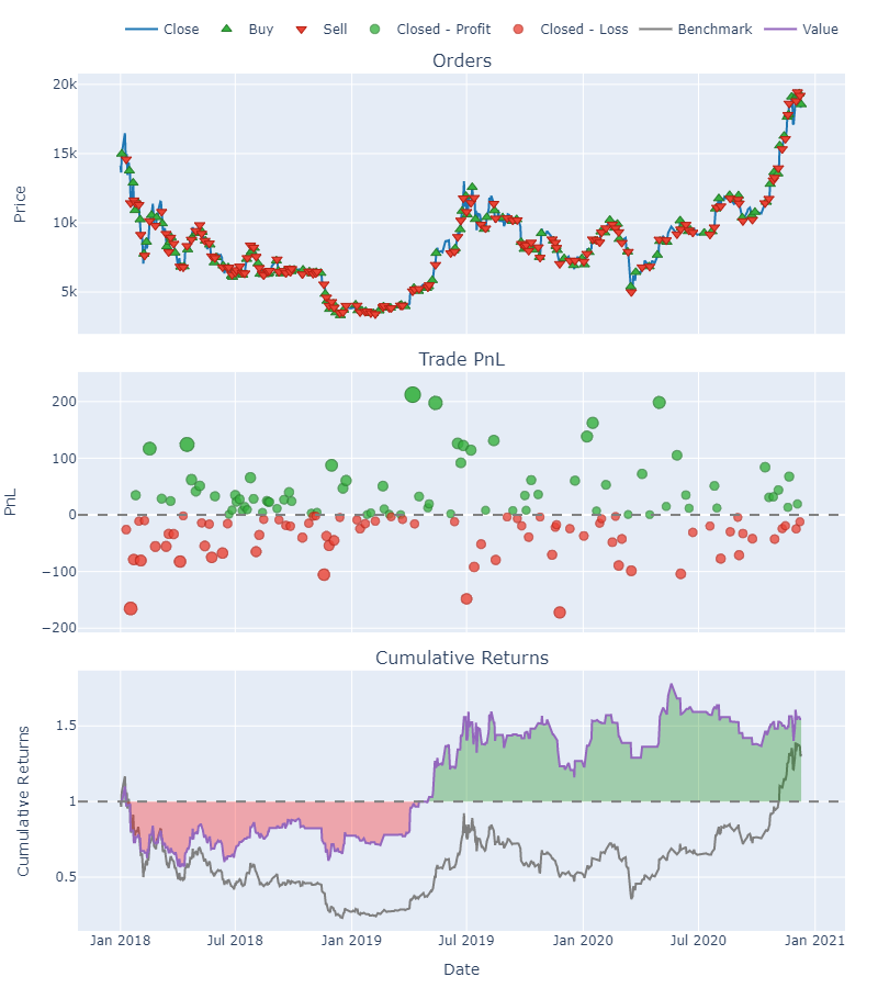
Start                           2018-01-01 00:00:00
End                             2020-12-10 00:00:00
Duration                          653 days 00:00:00
Init. Cash                                   1000.0
Total Profit                              546.37027
Total Return [%]                          54.637027
Benchmark Return [%]                      31.469924
Position Coverage [%]                     53.598775
Max. Drawdown [%]                         48.250763
Avg. Drawdown [%]                         14.777709
Max. Drawdown Duration            345 days 00:00:00
Avg. Drawdown Duration             63 days 21:36:00
Num. Trades                                     154
Win Rate [%]                                   50.0
Best Trade [%]                            27.551075
Worst Trade [%]                          -16.969197
Avg. Trade [%]                             0.468629
Max. Trade Duration                12 days 00:00:00
Avg. Trade Duration       2 days 06:23:22.597402597
Expectancy                                 3.547859
SQN                                        0.711113
Gross Exposure                             0.535988
Sharpe Ratio                                0.69902
Sortino Ratio                              1.059683
Calmar Ratio                               0.571815
Save and Load Model
trainer.save_checkpoint("bert.ckpt")
bert_reload = BERTBaseUncased.load_from_checkpoint(
    "bert.ckpt",
    num_classes=Config.NUM_CLASSES
)
NLP based Indicators and Technical Indicators
To make a profitable strategy, multiple criteria of entry-and-exit signals are often combined to filter out false positive decisions. In this work, NLP based indicators and technical indicators are combined into one single entry-and-exit signal array with true/false value using logical operators. There are two operators that combine multiple true or false values into a single true/false value.
ANDoperator: returns true only if both values are true.ORoperator: returns true when one of the values is true.
NLP based models are trained to predict whether the trend of the price is increasing or decreasing. Next, NLP based indicators are constructed by some trading rules as follow:
- If the forecast on
T-1day is “down-trend” and the forecast onTday is “up-trend”, then “buy” the open price onT+1day. - If the forecast on
T-1day is “up-trend” and the forecast onTday is “down-trend”, then “sell” the open price onT+1day. - If continue forecasting “up-trend”, then keep holding with the long-position.
- If continue forecasting “down-trend”, then keep holding without any long-position.
There are two basic types oftechnical indicators: Overlay Indicators and Oscillator Indicators.
In this project, only AND operator is used to set the condition to two criteria (NLP based indicators and technical indicators). For example, the entry signal is triggered when the RSI is above 50 and the NLP based indicator is producing a buy signal.
Relative Strength Index (RSI)
The Stochastic RSI (StochRSI) is a technical analysis indicator that ranges from 0 to 1 (or 0 to 100 on some charting platforms). It is calculated by applying the Stochastic oscillator formula to a collection of relative strength indexes (RSI). Overbought is defined as a StochRSI value above 0.8, while oversold is defined as a reading below 0.2. On the zero to 100 scale, above 80 is overbought, and below 20 is oversold.
price_test = text_price_df.iloc[-X_test.shape[0]:]
close = price_test.close
rsi = talib.RSI(close, timeperiod=14)
rsi.plot()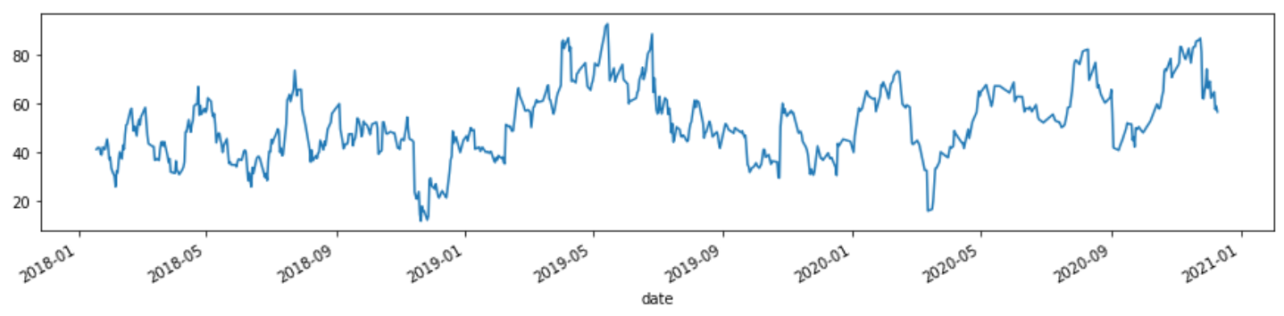
mlbp_rsi = MachineLearningBacktestPortfolio(price_test.open,
                                            entries=(rsi>=50).values&entries,
                                            exits=exits,
                                            show=True)
mlbp_rsi.plot_risk(figsize=(15, 10))
TextCNN and RSI
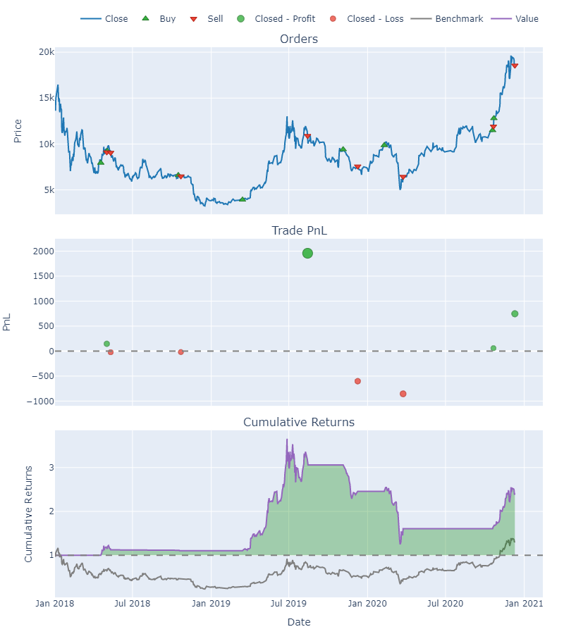
Start                            2018-01-01 00:00:00
End                              2020-12-10 00:00:00
Duration                           653 days 00:00:00
Init. Cash                                    1000.0
Total Profit                             1410.484857
Total Return [%]                          141.048486
Benchmark Return [%]                       31.469924
Position Coverage [%]                      30.015314
Max. Drawdown [%]                          65.917264
Avg. Drawdown [%]                           8.716855
Max. Drawdown Duration             272 days 00:00:00
Avg. Drawdown Duration    39 days 05:08:34.285714286
Num. Trades                                        8
Win Rate [%]                                    50.0
Best Trade [%]                            177.321644
Worst Trade [%]                           -34.745424
Avg. Trade [%]                             22.796415
Max. Trade Duration                 99 days 00:00:00
Avg. Trade Duration                 24 days 12:00:00
Expectancy                                176.310607
SQN                                         0.575284
Gross Exposure                              0.300153
Sharpe Ratio                                1.160131
Sortino Ratio                               1.730172
Calmar Ratio                                0.963688
BERT and RSI
Start                           2018-01-01 00:00:00
End                             2020-12-10 00:00:00
Duration                          653 days 00:00:00
Init. Cash                                   1000.0
Total Profit                            1372.905056
Total Return [%]                         137.290506
Benchmark Return [%]                      31.469924
Position Coverage [%]                     25.267994
Max. Drawdown [%]                         21.791524
Avg. Drawdown [%]                          6.460679
Max. Drawdown Duration            164 days 00:00:00
Avg. Drawdown Duration             32 days 01:20:00
Num. Trades                                      69
Win Rate [%]                              56.521739
Best Trade [%]                            27.551075
Worst Trade [%]                            -9.51275
Avg. Trade [%]                             1.430394
Max. Trade Duration                12 days 00:00:00
Avg. Trade Duration       2 days 09:02:36.521739130
Expectancy                                19.897175
SQN                                         1.63859
Gross Exposure                              0.25268
Sharpe Ratio                               1.309545
Sortino Ratio                              2.280386
Calmar Ratio                               2.849444
Williams %R (WILLR)
The Williams %R, often known as the Williams Percent Range, is a sort of momentum indicator that monitors overbought and oversold conditions and travels between 0 and -100. The Williams %R can be used to determine market entrance and exit points. A reading of -20 indicates that the market is overbought. A value of -80 indicates that the market is oversold.
high = price_test.high
low = price_test.low
close = price_test.close
willr = talib.WILLR(high, low, close, timeperiod=14)
willr.plot()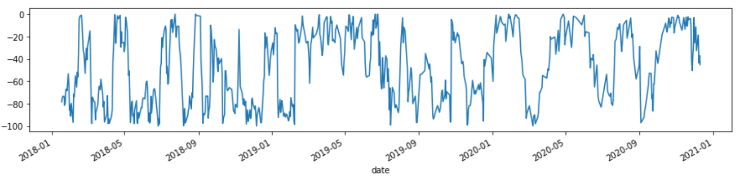
mlbp_willr = MachineLearningBacktestPortfolio(price_test.open,
                                              entries=(willr>=-40).values&entries,
                                              exits=exits,
                                              show=True)
mlbp_willr.plot_risk(figsize=(15, 10))
TextCNN and WILLR

Start 2018-01-01 00:00:00
End 2020-12-10 00:00:00
Duration 653 days 00:00:00
Init. Cash 1000.0
Total Profit 1197.129932
Total Return [%] 119.712993
Benchmark Return [%] 31.469924
Position Coverage [%] 36.600306
Max. Drawdown [%] 65.917264
Avg. Drawdown [%] 11.492131
Max. Drawdown Duration 272 days 00:00:00
Avg. Drawdown Duration 42 days 07:23:04.615384615
Num. Trades 9
Win Rate [%] 44.444444
Best Trade [%] 177.321644
Worst Trade [%] -34.745424
Avg. Trade [%] 19.2688
Max. Trade Duration 99 days 00:00:00
Avg. Trade Duration 26 days 13:20:00
Expectancy 133.014437
SQN 0.536334
Gross Exposure 0.366003
Sharpe Ratio 1.038628
Sortino Ratio 1.546713
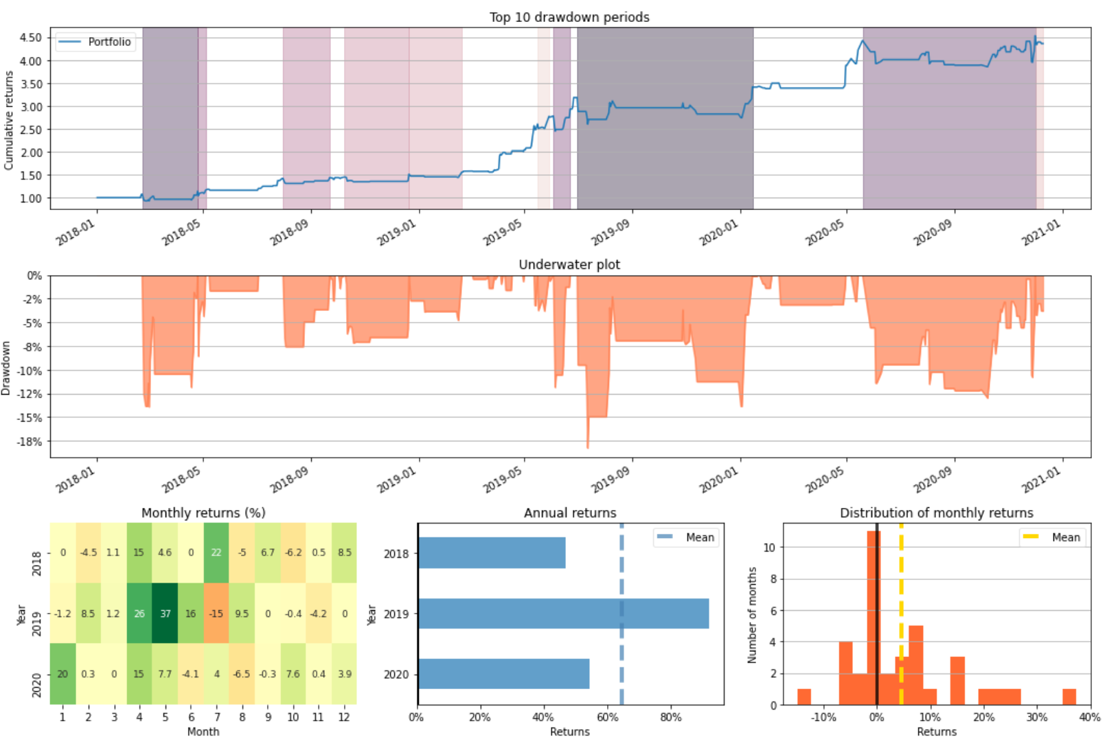
Calmar Ratio 0.838452BERT and WILLR
Start                            2018-01-01 00:00:00
End                              2020-12-10 00:00:00
Duration                           653 days 00:00:00
Init. Cash                                    1000.0
Total Profit                             3817.273877
Total Return [%]                          381.727388
Benchmark Return [%]                       31.469924
Position Coverage [%]                      21.898928
Max. Drawdown [%]                          13.930189
Avg. Drawdown [%]                           4.238248
Max. Drawdown Duration             138 days 00:00:00
Avg. Drawdown Duration    21 days 10:54:32.727272727
Num. Trades                                       60
Win Rate [%]                                    70.0
Best Trade [%]                             27.551075
Worst Trade [%]                            -7.566861
Avg. Trade [%]                              2.823779
Max. Trade Duration                 12 days 00:00:00
Avg. Trade Duration                  2 days 09:12:00
Expectancy                                 63.621231
SQN                                         3.163193
Gross Exposure                              0.218989
Sharpe Ratio                                2.360838
Sortino Ratio                               4.953118
Calmar Ratio                               10.107593
Aroon Oscillator (AROONOSC)
The Aroon indicator is a technical indicator that may be used to detect price trend changes as well as the strength of that trend. In essence, the indicator calculates the time between highs and lows over a given period of time. The notion is that strong uptrends will see new highs on a frequent basis, whereas strong downtrends would see new lows on a frequent basis.
high = price_test.high
low = price_test.low
aroonosc = talib.AROONOSC(high, low, timeperiod=14)
aroonosc.plot()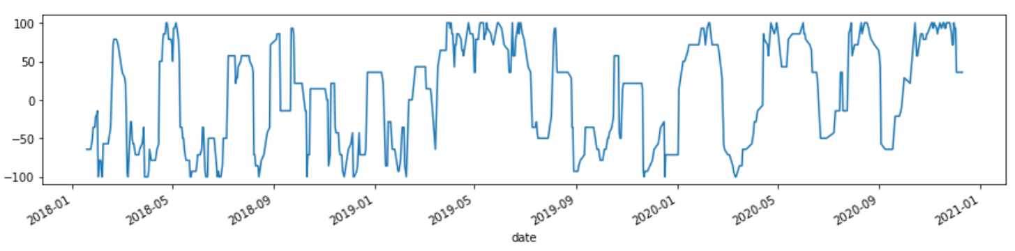
mlbp_aroonosc = MachineLearningBacktestPortfolio(price_test.open,
                                                 entries=(aroonosc>=25).values&entries,
                                                 exits=exits,
                                                 show=True)
mlbp_aroonosc.plot_risk(figsize=(15, 10))
TextCNN and AROONOSC
Start                     2018-01-01 00:00:00
End                       2020-12-10 00:00:00
Duration                    653 days 00:00:00
Init. Cash                             1000.0
Total Profit                        58.852402
Total Return [%]                      5.88524
Benchmark Return [%]                31.469924
Position Coverage [%]               16.385911
Max. Drawdown [%]                   60.573478
Avg. Drawdown [%]                   17.173099
Max. Drawdown Duration      494 days 00:00:00
Avg. Drawdown Duration      112 days 09:36:00
Num. Trades                                 8
Win Rate [%]                             62.5
Best Trade [%]                      44.929126
Worst Trade [%]                    -34.745424
Avg. Trade [%]                       2.854736
Max. Trade Duration          33 days 00:00:00
Avg. Trade Duration          13 days 09:00:00
Expectancy                            7.35655
SQN                                  0.104441
Gross Exposure                       0.163859
Sharpe Ratio                         0.301499
Sortino Ratio                        0.397515
Calmar Ratio                         0.053622
BERT and AROONOSC
Start                            2018-01-01 00:00:00
End                              2020-12-10 00:00:00
Duration                           653 days 00:00:00
Init. Cash                                    1000.0
Total Profit                             1411.933816
Total Return [%]                          141.193382
Benchmark Return [%]                       31.469924
Position Coverage [%]                      22.205207
Max. Drawdown [%]                          23.302887
Avg. Drawdown [%]                           6.746358
Max. Drawdown Duration             164 days 00:00:00
Avg. Drawdown Duration    30 days 07:34:44.210526315
Num. Trades                                       70
Win Rate [%]                               57.142857
Best Trade [%]                             27.551075
Worst Trade [%]                             -9.51275
Avg. Trade [%]                              1.430573
Max. Trade Duration                 12 days 00:00:00
Avg. Trade Duration        2 days 01:22:17.142857142
Expectancy                                 20.170483
SQN                                          1.70467
Gross Exposure                              0.222052
Sharpe Ratio                                1.403516
Sortino Ratio                               2.525902
Calmar Ratio                                2.728357
Balance Of Power (BOP)
Balance of Power (BOP) is an oscillator that measures the strength of buying and selling pressure. Introduced by Igor Levshin in the August 2001 issue of Technical Analysis of Stocks & Commodities magazine, this indicator compares the power of buyers to push prices to higher extremes with the power of sellers to move prices to lower extremes. When the indicator is in positive territory, the bulls are in charge; and sellers dominate when the indicator is negative. A reading near the zero line indicates a balance between the two and can mean a trend reversal.
open_ = price_test.open
high = price_test.high
low = price_test.low
close = price_test.close
bop = talib.BOP(open_, high, low, close)
bop.plot()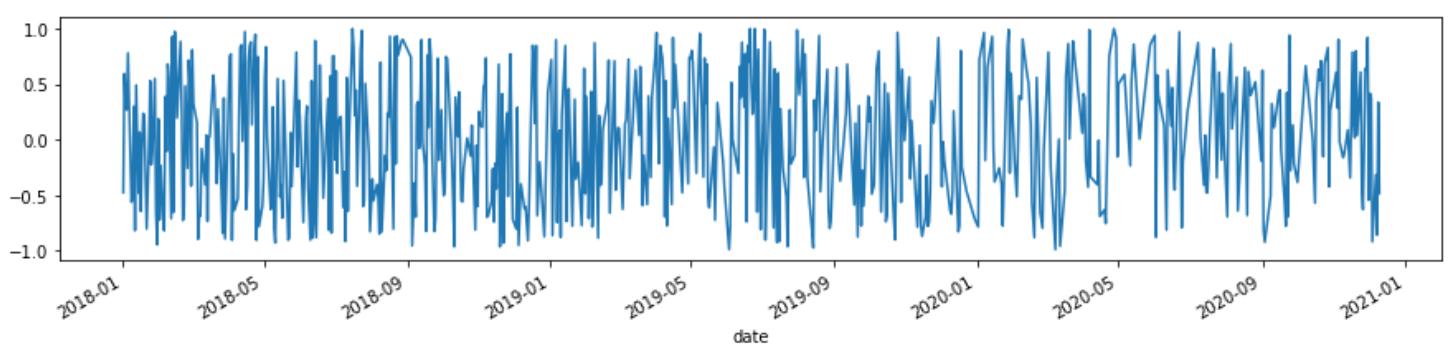
mlbp_bop = MachineLearningBacktestPortfolio(price_test.open,
                                            entries=(bop>=0.8).values&entries,
                                            exits=exits,
                                            show=True)
mlbp_bop.plot_risk(figsize=(15, 10))
TextCNN and BOP
Start                     2018-01-01 00:00:00
End                       2020-12-10 00:00:00
Duration                    653 days 00:00:00
Init. Cash                             1000.0
Total Profit                       -387.11781
Total Return [%]                   -38.711781
Benchmark Return [%]                31.469924
Position Coverage [%]                 9.49464
Max. Drawdown [%]                   58.149854
Avg. Drawdown [%]                   33.387792
Max. Drawdown Duration      469 days 00:00:00
Avg. Drawdown Duration      276 days 12:00:00
Num. Trades                                 4
Win Rate [%]                              0.0
Best Trade [%]                      -0.620421
Worst Trade [%]                    -34.745424
Avg. Trade [%]                     -10.232098
Max. Trade Duration          22 days 00:00:00
Avg. Trade Duration          15 days 12:00:00
Expectancy                         -96.779453
SQN                                 -1.261007
Gross Exposure                       0.094946
Sharpe Ratio                        -0.546112
Sortino Ratio                       -0.662911
Calmar Ratio                        -0.411706
BERT and BOP
Start                           2018-01-01 00:00:00
End                             2020-12-10 00:00:00
Duration                          653 days 00:00:00
Init. Cash                                   1000.0
Total Profit                             852.560933
Total Return [%]                          85.256093
Benchmark Return [%]                      31.469924
Position Coverage [%]                      3.675345
Max. Drawdown [%]                         13.856424
Avg. Drawdown [%]                          7.633348
Max. Drawdown Duration            139 days 00:00:00
Avg. Drawdown Duration             82 days 00:00:00
Num. Trades                                      11
Win Rate [%]                              90.909091
Best Trade [%]                            21.832492
Worst Trade [%]                           -7.165814
Avg. Trade [%]                             5.996617
Max. Trade Duration                 5 days 00:00:00
Avg. Trade Duration       2 days 04:21:49.090909090
Expectancy                                77.505539
SQN                                        3.051468
Gross Exposure                             0.036753
Sharpe Ratio                               1.699568
Sortino Ratio                              3.867465
Calmar Ratio                               2.969575
Market Meanness Index (MMI)
The Market Meanness Index tells whether the market is currently moving in or out of a ‘trending’ regime. It can this way prevent losses by false signals of trend indicators. It is a purely statisticalalgorithm and not based on volatility, trends, or cycles of the price curve.
mmi_days = 20
close = price_test.close
median = close.rolling(mmi_days).median()
p1 = close>median
p2 = close.shift() > median
mmi = (p1 & p2).astype(int).rolling(mmi_days).mean()
mmi.plot()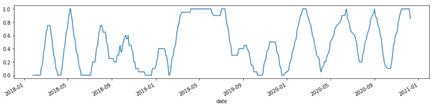
mlbp_mmi = MachineLearningBacktestPortfolio(price_test.open,
                                            entries=(mmi>=0.5).values&entries,
                                            exits=exits,
                                            show=True)
mlbp_mmi.plot_risk(figsize=(15, 10))
TextCNN and MMI
Start                            2018-01-01 00:00:00
End                              2020-12-10 00:00:00
Duration                           653 days 00:00:00
Init. Cash                                    1000.0
Total Profit                              164.578985
Total Return [%]                           16.457898
Benchmark Return [%]                       31.469924
Position Coverage [%]                      28.024502
Max. Drawdown [%]                           57.57344
Avg. Drawdown [%]                          17.096136
Max. Drawdown Duration             294 days 00:00:00
Avg. Drawdown Duration    83 days 17:08:34.285714285
Num. Trades                                        7
Win Rate [%]                               14.285714
Best Trade [%]                            177.321644
Worst Trade [%]                           -34.745424
Avg. Trade [%]                             14.702369
Max. Trade Duration                 99 days 00:00:00
Avg. Trade Duration       26 days 03:25:42.857142857
Expectancy                                 23.511284
SQN                                         0.115111
Gross Exposure                              0.280245
Sharpe Ratio                                0.445331
Sortino Ratio                               0.622654
Calmar Ratio                                0.154401
BERT and MMI
Start                     2018-01-01 00:00:00
End                       2020-12-10 00:00:00
Duration                    653 days 00:00:00
Init. Cash                             1000.0
Total Profit                        -61.14569
Total Return [%]                    -6.114569
Benchmark Return [%]                31.469924
Position Coverage [%]               24.808576
Max. Drawdown [%]                   47.765242
Avg. Drawdown [%]                   13.595813
Max. Drawdown Duration      299 days 00:00:00
Avg. Drawdown Duration       74 days 12:00:00
Num. Trades                                69
Win Rate [%]                        42.028986
Best Trade [%]                      27.551075
Worst Trade [%]                    -12.259609
Avg. Trade [%]                        0.08213
Max. Trade Duration          12 days 00:00:00
Avg. Trade Duration           2 days 08:00:00
Expectancy                          -0.886169
SQN                                 -0.113694
Gross Exposure                       0.248086
Sharpe Ratio                         0.125302
Sortino Ratio                        0.199014
Calmar Ratio                        -0.072548
Commodity Channel Index (CCI)
The Commodity Channel Index (CCI) is a momentum-based oscillator used to help determine when an investment vehicle is reaching a condition of being overbought or oversold. When the CCI is above zero, it indicates the price is above the historic average. Conversely, when the CCI is below zero, the price is below the historic average.
high = price_test.high
low = price_test.low
close = price_test.close
cci = talib.CCI(high, low, close, timeperiod=14)
cci.plot()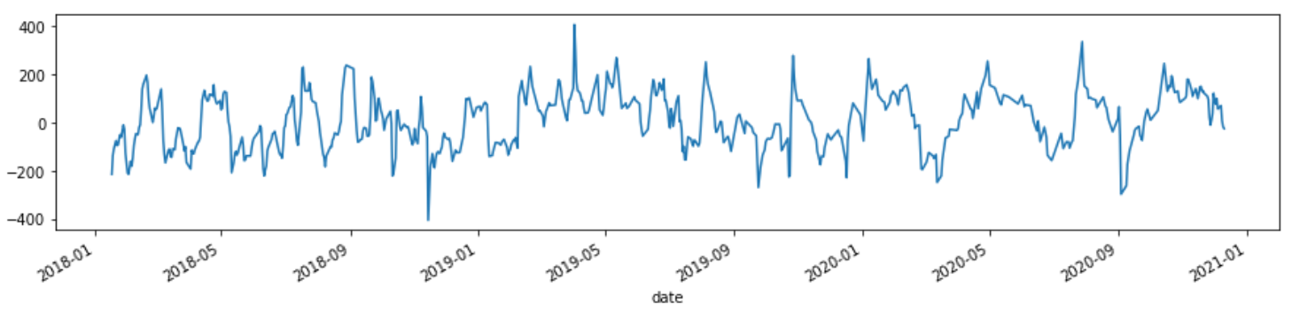
mlbp_cci = MachineLearningBacktestPortfolio(price_test.open,
                                            entries=(cci>=0).values&entries,
                                            exits=exits,
                                            show=True)
mlbp_cci.plot_risk(figsize=(15, 10))
TextCNN and CCI
Start                            2018-01-01 00:00:00
End                              2020-12-10 00:00:00
Duration                           653 days 00:00:00
Init. Cash                                    1000.0
Total Profit                             1158.734851
Total Return [%]                          115.873485
Benchmark Return [%]                       31.469924
Position Coverage [%]                      37.212864
Max. Drawdown [%]                          65.917264
Avg. Drawdown [%]                          11.588112
Max. Drawdown Duration             272 days 00:00:00
Avg. Drawdown Duration    42 days 07:23:04.615384615
Num. Trades                                       10
Win Rate [%]                                    40.0
Best Trade [%]                            177.321644
Worst Trade [%]                           -34.745424
Avg. Trade [%]                             17.167169
Max. Trade Duration                 99 days 00:00:00
Avg. Trade Duration                 24 days 07:12:00
Expectancy                                115.873485
SQN                                         0.530371
Gross Exposure                              0.372129
Sharpe Ratio                                1.022194
Sortino Ratio                               1.522095
Calmar Ratio                                0.815354
BERT and CCI
Start                           2018-01-01 00:00:00
End                             2020-12-10 00:00:00
Duration                          653 days 00:00:00
Init. Cash                                   1000.0
Total Profit                            3357.754498
Total Return [%]                          335.77545
Benchmark Return [%]                      31.469924
Position Coverage [%]                     26.799387
Max. Drawdown [%]                         18.274166
Avg. Drawdown [%]                          4.626804
Max. Drawdown Duration            110 days 00:00:00
Avg. Drawdown Duration             21 days 21:07:12
Num. Trades                                      73
Win Rate [%]                              64.383562
Best Trade [%]                            27.551075
Worst Trade [%]                            -9.51275
Avg. Trade [%]                             2.201906
Max. Trade Duration                12 days 00:00:00
Avg. Trade Duration       2 days 09:32:03.287671232
Expectancy                                45.996637
SQN                                        2.703271
Gross Exposure                             0.267994
Sharpe Ratio                               2.123362
Sortino Ratio                               4.15713
Calmar Ratio                               6.986814
Moving Average Convergence/Divergence (MACD)
Moving average convergence divergence (MACD) is a trend-following momentum indicator that shows the relationship between two moving averages of a security’s price. The MACD is calculated by subtracting the 26-period exponential moving average (EMA) from the 12-period EMA.
close = price_test.close
macd, macdsignal, macdhist = talib.MACD(close, fastperiod=12, slowperiod=26, signalperiod=9)
macd.plot()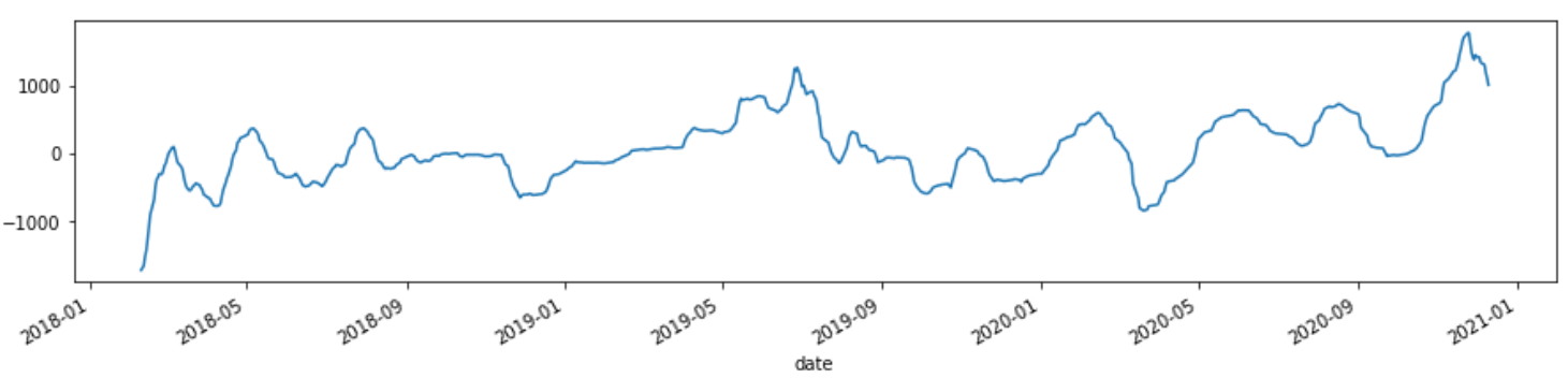
mlbp_macd = MachineLearningBacktestPortfolio(price_test.open,
                                             entries=(macd>=0).values&entries,
                                             exits=exits,
                                             show=True)
mlbp_macd.plot_risk(figsize=(15, 10))
TextCNN and MACD
Start                     2018-01-01 00:00:00
End                       2020-12-10 00:00:00
Duration                    653 days 00:00:00
Init. Cash                             1000.0
Total Profit                       990.617772
Total Return [%]                    99.061777
Benchmark Return [%]                31.469924
Position Coverage [%]               31.087289
Max. Drawdown [%]                   64.725467
Avg. Drawdown [%]                   10.406998
Max. Drawdown Duration      272 days 00:00:00
Avg. Drawdown Duration       44 days 22:00:00
Num. Trades                                 9
Win Rate [%]                        55.555556
Best Trade [%]                     177.321644
Worst Trade [%]                    -34.745424
Avg. Trade [%]                      18.092523
Max. Trade Duration          99 days 00:00:00
Avg. Trade Duration          22 days 13:20:00
Expectancy                         110.068641
SQN                                  0.501126
Gross Exposure                       0.310873
Sharpe Ratio                         0.969612
Sortino Ratio                        1.428536
Calmar Ratio                         0.725122
BERT and MACD
Start                     2018-01-01 00:00:00
End                       2020-12-10 00:00:00
Duration                    653 days 00:00:00
Init. Cash                             1000.0
Total Profit                       501.301519
Total Return [%]                    50.130152
Benchmark Return [%]                31.469924
Position Coverage [%]               21.133231
Max. Drawdown [%]                   35.199714
Avg. Drawdown [%]                    8.540103
Max. Drawdown Duration      266 days 00:00:00
Avg. Drawdown Duration       44 days 18:00:00
Num. Trades                                64
Win Rate [%]                             50.0
Best Trade [%]                      27.551075
Worst Trade [%]                      -9.51275
Avg. Trade [%]                       0.792115
Max. Trade Duration          12 days 00:00:00
Avg. Trade Duration           2 days 03:22:30
Expectancy                           7.832836
SQN                                  0.779408
Gross Exposure                       0.211332
Sharpe Ratio                         0.756469
Sortino Ratio                        1.262302
Calmar Ratio                         0.724393
Money Flow Index (MFI)
The Money Flow Index (MFI) is a technical oscillator that uses price and volume data for identifying overbought or oversold signals in an asset. It can also be used to spot divergences which warn of a trend change in price. The oscillator moves between 0 and 100. Unlike conventional oscillators such as the Relative Strength Index (RSI), the Money Flow Index incorporates both price and volume data, as opposed to just price. For this reason, some analysts call MFI the volume-weighted RSI.
high = price_test.high
low = price_test.low
close = price_test.close
volume = price_test.volume
mfi = talib.MFI(high, low, close, volume, timeperiod=14)
mfi.plot()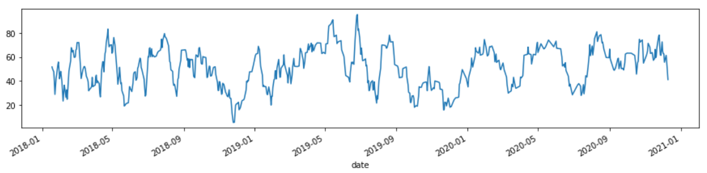
mlbp_mfi = MachineLearningBacktestPortfolio(price_test.open,
                                            entries=(mfi>=50).values&entries,
                                            exits=exits,
                                            show=True)
mlbp_mfi.plot_risk(figsize=(15, 10))
TextCNN and MFI
Start                            2018-01-01 00:00:00
End                              2020-12-10 00:00:00
Duration                           653 days 00:00:00
Init. Cash                                    1000.0
Total Profit                              543.096364
Total Return [%]                           54.309636
Benchmark Return [%]                       31.469924
Position Coverage [%]                      39.356815
Max. Drawdown [%]                          65.619075
Avg. Drawdown [%]                          15.958521
Max. Drawdown Duration             272 days 00:00:00
Avg. Drawdown Duration              55 days 04:48:00
Num. Trades                                       13
Win Rate [%]                               46.153846
Best Trade [%]                            177.321644
Worst Trade [%]                           -34.745424
Avg. Trade [%]                             11.136054
Max. Trade Duration                 99 days 00:00:00
Avg. Trade Duration       19 days 18:27:41.538461538
Expectancy                                 41.776643
SQN                                         0.338795
Gross Exposure                              0.393568
Sharpe Ratio                                0.710413
Sortino Ratio                               1.016296
Calmar Ratio                                0.418163
BERT and MFI
Start                            2018-01-01 00:00:00
End                              2020-12-10 00:00:00
Duration                           653 days 00:00:00
Init. Cash                                    1000.0
Total Profit                              755.505657
Total Return [%]                           75.550566
Benchmark Return [%]                       31.469924
Position Coverage [%]                      28.024502
Max. Drawdown [%]                          21.682457
Avg. Drawdown [%]                           8.642257
Max. Drawdown Duration             164 days 00:00:00
Avg. Drawdown Duration    43 days 06:51:25.714285714
Num. Trades                                       81
Win Rate [%]                                53.08642
Best Trade [%]                             27.551075
Worst Trade [%]                             -9.51275
Avg. Trade [%]                               0.84668
Max. Trade Duration                 12 days 00:00:00
Avg. Trade Duration        2 days 06:13:19.999999999
Expectancy                                   9.32723
SQN                                         1.140512
Gross Exposure                              0.280245
Sharpe Ratio                                0.943201
Sortino Ratio                               1.598255
Calmar Ratio                                1.704851
Momentum (MOM)
The Momentum Indicator (MOM) is a leading indicator measuring a security’s rate-of-change. It compares the current price with the previous price from a number of periods ago.The ongoing plot forms an oscillator that moves above and below 0. It is a fully unbounded oscillator and has no lower or upper limit. Bullish and bearish interpretations are found by looking for divergences, centerline crossovers and extreme readings. The indicator is often used in combination with other signals.
close = price_test.close
mom = talib.MOM(close, timeperiod=10)
mom.plot()
mlbp_mom = MachineLearningBacktestPortfolio(price_test.open,
                                            entries=(mom>=0).values&entries,
                                            exits=exits,
                                            show=True)
mlbp_mom.plot_risk(figsize=(15, 10))
TextCNN and MOM
Start                            2018-01-01 00:00:00
End                              2020-12-10 00:00:00
Duration                           653 days 00:00:00
Init. Cash                                    1000.0
Total Profit                              889.771213
Total Return [%]                           88.977121
Benchmark Return [%]                       31.469924
Position Coverage [%]                      42.113323
Max. Drawdown [%]                          65.563822
Avg. Drawdown [%]                           12.87516
Max. Drawdown Duration             272 days 00:00:00
Avg. Drawdown Duration              55 days 04:48:00
Num. Trades                                       13
Win Rate [%]                               38.461538
Best Trade [%]                            177.321644
Worst Trade [%]                           -34.745424
Avg. Trade [%]                             12.246031
Max. Trade Duration                 99 days 00:00:00
Avg. Trade Duration       21 days 03:41:32.307692307
Expectancy                                 68.443939
SQN                                         0.469819
Gross Exposure                              0.421133
Sharpe Ratio                                0.891946
Sortino Ratio                               1.312906
Calmar Ratio                                0.651662
BERT and MOM
Start                     2018-01-01 00:00:00
End                       2020-12-10 00:00:00
Duration                    653 days 00:00:00
Init. Cash                             1000.0
Total Profit                       1759.54364
Total Return [%]                   175.954364
Benchmark Return [%]                31.469924
Position Coverage [%]               28.177642
Max. Drawdown [%]                   20.780414
Avg. Drawdown [%]                    7.379898
Max. Drawdown Duration      116 days 00:00:00
Avg. Drawdown Duration       29 days 12:00:00
Num. Trades                                75
Win Rate [%]                        57.333333
Best Trade [%]                      27.551075
Worst Trade [%]                    -12.763619
Avg. Trade [%]                       1.539368
Max. Trade Duration          12 days 00:00:00
Avg. Trade Duration           2 days 10:33:36
Expectancy                          23.460582
SQN                                  2.002748
Gross Exposure                       0.281776
Sharpe Ratio                         1.466978
Sortino Ratio                         2.55946
Calmar Ratio                         3.674804
Ultimate Oscillator (ULTOSC)
The Ultimate Oscillator is a technical indicator that was developed by Larry Williams in 1976 to measure the price momentum of an asset across multiple timeframes. By using the weighted average of three different timeframes the indicator has less volatility and fewer trade signals compared to other oscillators that rely on a single timeframe. Buy and sell signals are generated following divergences. The Ultimately Oscillator generates fewer divergence signals than other oscillators due to its multi-timeframe construction. Buy signals occur when there is bullish divergence, the divergence low is below 30 on the indicator, and the oscillator then rises above the divergence high. A sell signal occurs when there is bearish divergence, the divergence high is above 70, and the oscillator then falls below the divergence low.
high = price_test.high
low = price_test.low
close = price_test.close
ultosc = talib.ULTOSC(high, low, close, timeperiod1=7, timeperiod2=14, timeperiod3=28)
ultosc.plot()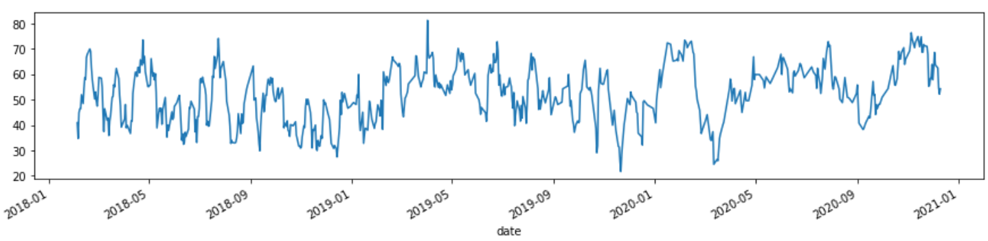
mlbp_ultosc = MachineLearningBacktestPortfolio(price_test.open,
                                               entries=(ultosc>=50).values&entries,
                                               exits=exits,
                                               show=True)
mlbp_ultosc.plot_risk(figsize=(15, 10))
TextCNN and ULTOSC
Start                            2018-01-01 00:00:00
End                              2020-12-10 00:00:00
Duration                           653 days 00:00:00
Init. Cash                                    1000.0
Total Profit                             2438.525894
Total Return [%]                          243.852589
Benchmark Return [%]                       31.469924
Position Coverage [%]                      58.499234
Max. Drawdown [%]                          69.323364
Avg. Drawdown [%]                          10.761178
Max. Drawdown Duration             255 days 00:00:00
Avg. Drawdown Duration              34 days 06:00:00
Num. Trades                                       14
Win Rate [%]                                    50.0
Best Trade [%]                            177.321644
Worst Trade [%]                           -34.745424
Avg. Trade [%]                             17.228297
Max. Trade Duration                 99 days 00:00:00
Avg. Trade Duration       27 days 06:51:25.714285714
Expectancy                                174.180421
SQN                                         0.959201
Gross Exposure                              0.584992
Sharpe Ratio                                1.341326
Sortino Ratio                               2.085091
Calmar Ratio                                1.434422
BERT and ULTOSC
Start                            2018-01-01 00:00:00
End                              2020-12-10 00:00:00
Duration                           653 days 00:00:00
Init. Cash                                    1000.0
Total Profit                             1885.787803
Total Return [%]                           188.57878
Benchmark Return [%]                       31.469924
Position Coverage [%]                      28.177642
Max. Drawdown [%]                          17.968363
Avg. Drawdown [%]                           6.135872
Max. Drawdown Duration             145 days 00:00:00
Avg. Drawdown Duration    26 days 21:42:51.428571428
Num. Trades                                       77
Win Rate [%]                               57.142857
Best Trade [%]                             27.551075
Worst Trade [%]                             -9.51275
Avg. Trade [%]                              1.541911
Max. Trade Duration                 12 days 00:00:00
Avg. Trade Duration        2 days 09:02:20.259740259
Expectancy                                 24.490751
SQN                                          2.06409
Gross Exposure                              0.281776
Sharpe Ratio                                1.544248
Sortino Ratio                               2.746532
Calmar Ratio                                4.498422
Performance
The total return is -27.1728% if only the TextCNN model is used to produce buy-and-sell signals. After using various technical indicators to filter out false negative signals, all average drawdowns are smaller than when using TextCNN alone.
Ten different technical indicators are deployed as filters in this project. Only BOP produces a worse Sharpe Ratio when utilising technical indicators as filters than when using TextCNN alone; on the other hand, the other 9 technical indicators produce a higher Sharpe Ratio score. However, the maximum drawdown is higher when utilising technical indicators as filters than when using TextCNN alone for all technical indicators.
| Technical Indicator | Total Return [%] | Max. Drawdown [%] | Avg. Drawdown [%] | Sharpe Ratio |
|---|---|---|---|---|
| TextCNN | -27.1728 | 52.8665 | 26.4332 | -0.4187 |
| TextCNN + RSI | 141.0484 | 65.9172 | 8.7168 | 1.1601 |
| TextCNN + WILLR | 119.7129 | 65.9172 | 11.4921 | 1.0386 |
| TextCNN + AROONOSC | 5.8852 | 60.5734 | 17.1731 | 0.3014 |
| TextCNN + BOP | -38.7117 | 58.1498 | 33.3877 | -0.5461 |
| TextCNN + MMI | 16.4578 | 57.5734 | 17.0961 | 0.4453 |
| TextCNN + CCI | 115.8734 | 65.9172 | 11.5881 | 1.0221 |
| TextCNN + MACD | 99.0617 | 64.7254 | 10.4069 | 0.9696 |
| TextCNN + MFI | 54.3096 | 65.6190 | 15.9585 | 0.7104 |
| TextCNN + MOM | 88.9771 | 65.5638 | 12.8751 | 0.8919 |
| TextCNN + ULTOSC | 243.8525 | 69.3233 | 10.7611 | 1.3413 |
BERT appears to produce a better outcome than TextCNN. Except for MMI, all of the indicators that integrate with BERT can have a total return of more than 50%. Despite having a negative total return of -6.1145, BERT + MMI has a positive Sharpe Ratio of 0.1253. When combining BERT and technical indicators, the maximum and average drawdowns are smaller than when using the language model alone, and the Sharpe Ratio are all positive. WILLR and CCI can even triple the total return compared to the original.
| Technical Indicator | Total Return [%] | Max. Drawdown [%] | Avg. Drawdown [%] | Sharpe Ratio |
|---|---|---|---|---|
| BERT | 54.6370 | 48.2507 | 14.7777 | 0.6990 |
| BERT + RSI | 137.2905 | 21.7915 | 6.4606 | 1.3095 |
| BERT + WILLR | 381.7274 | 13.9302 | 4.2382 | 2.3608 |
| BERT + AROONOSC | 141.1933 | 23.3028 | 6.7464 | 1.4035 |
| BERT + BOP | 85.2560 | 13.8564 | 7.6333 | 1.6996 |
| BERT + MMI | -6.1145 | 47.7652 | 13.5958 | 0.1253 |
| BERT + CCI | 335.7754 | 18.2741 | 4.6268 | 2.1233 |
| BERT + MACD | 50.1301 | 35.1997 | 8.5401 | 0.7564 |
| BERT + MFI | 75.5505 | 21.6824 | 8.6422 | 0.9432 |
| BERT + MOM | 175.9543 | 20.7804 | 7.3798 | 1.4669 |
| BERT + ULTOSC | 188.5787 | 17.9683 | 6.1358 | 1.5442 |
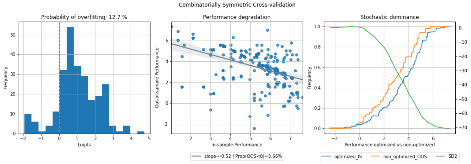
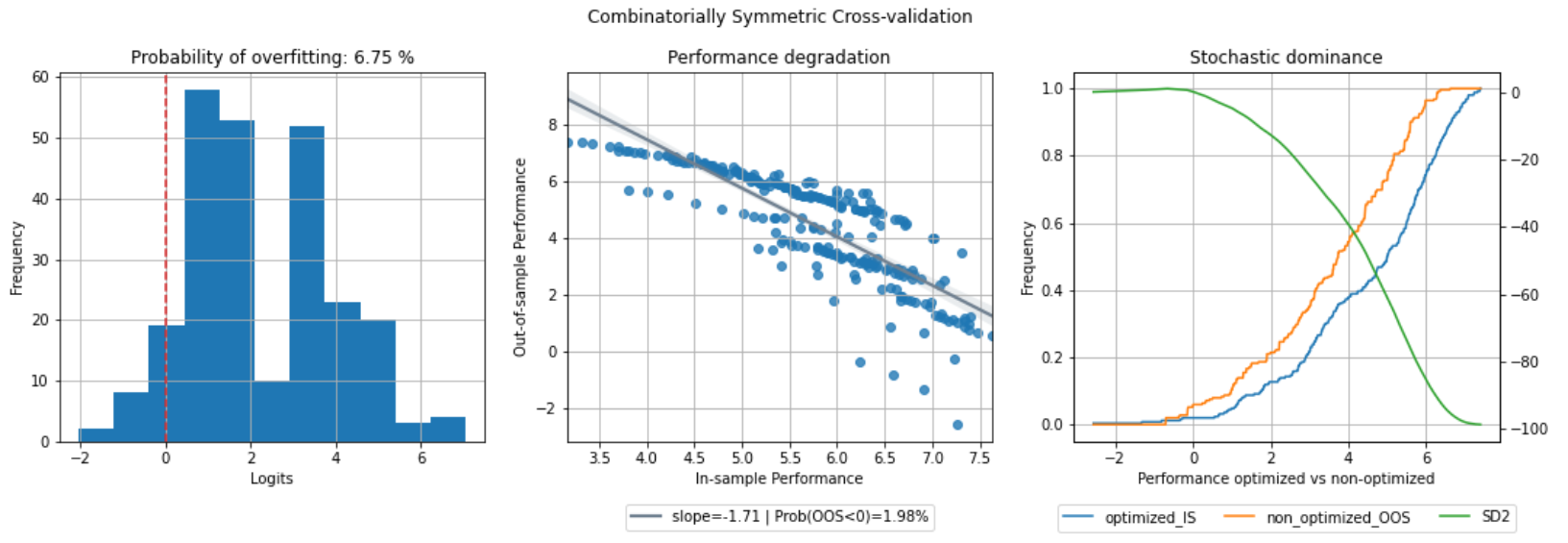
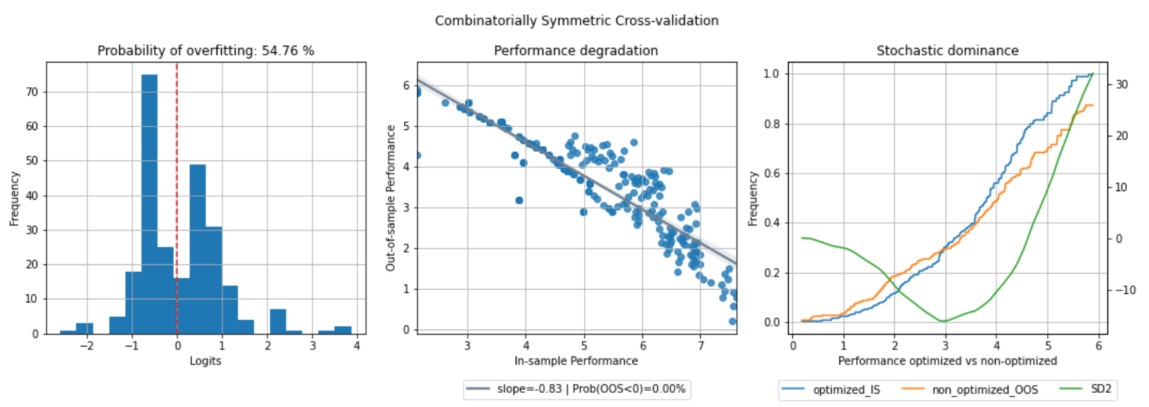
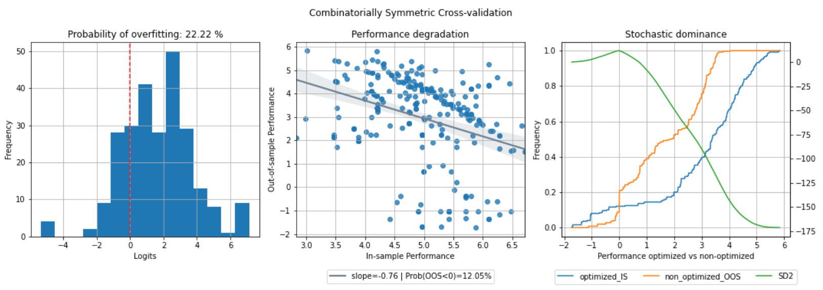
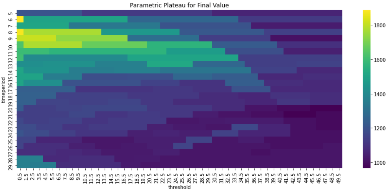
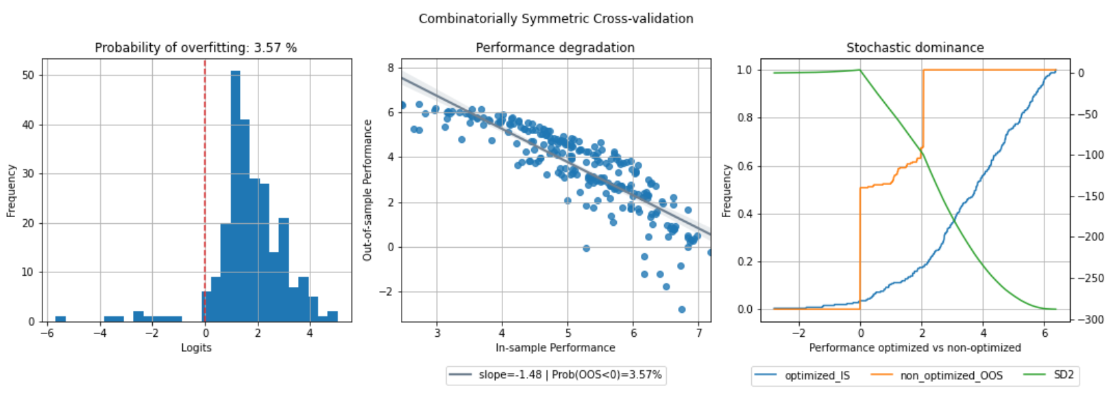
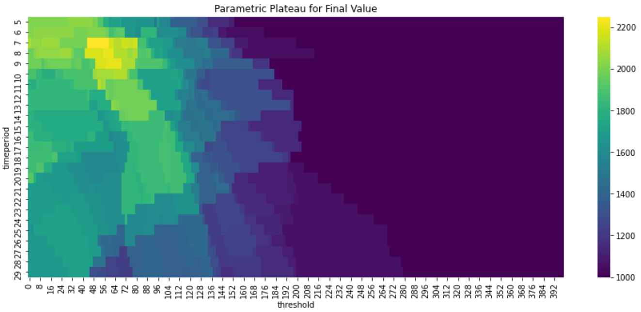
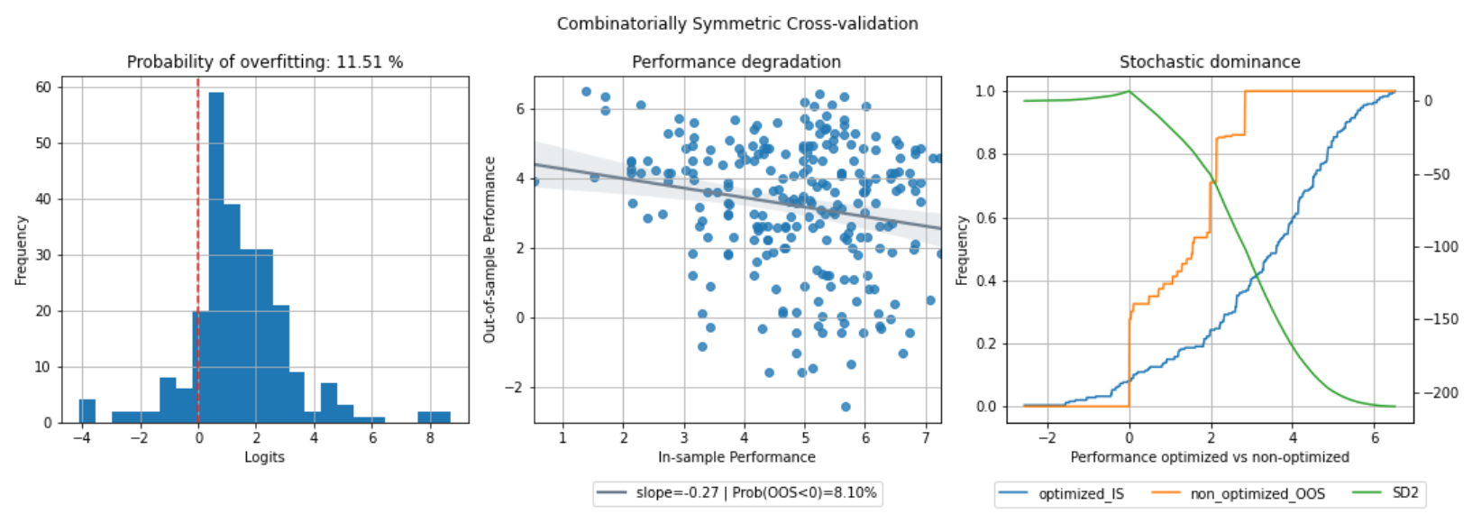
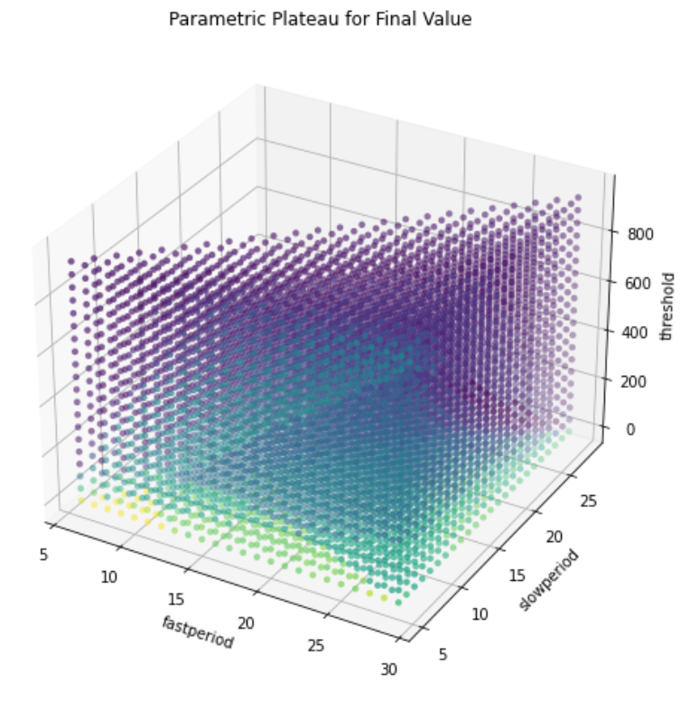
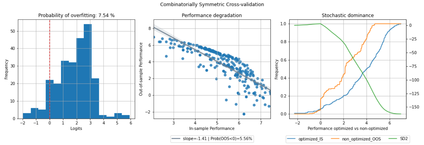
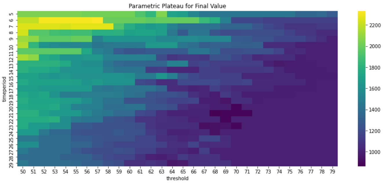
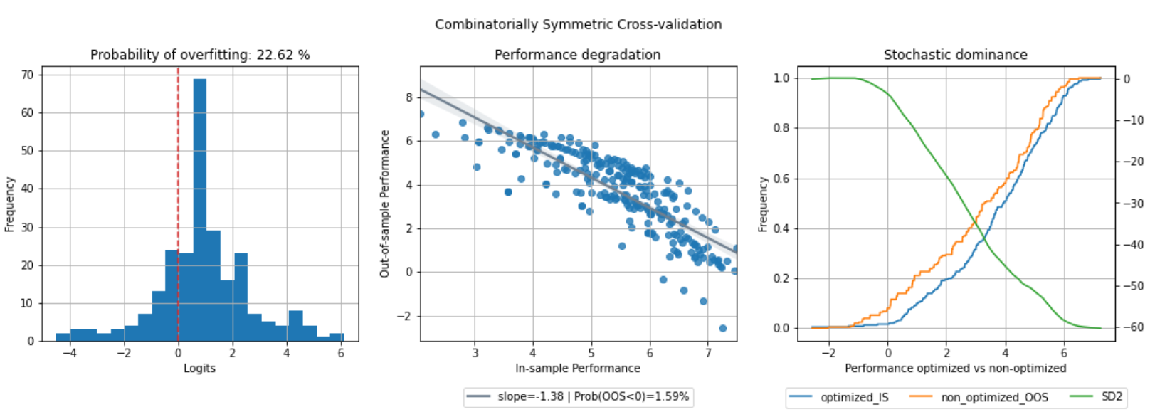
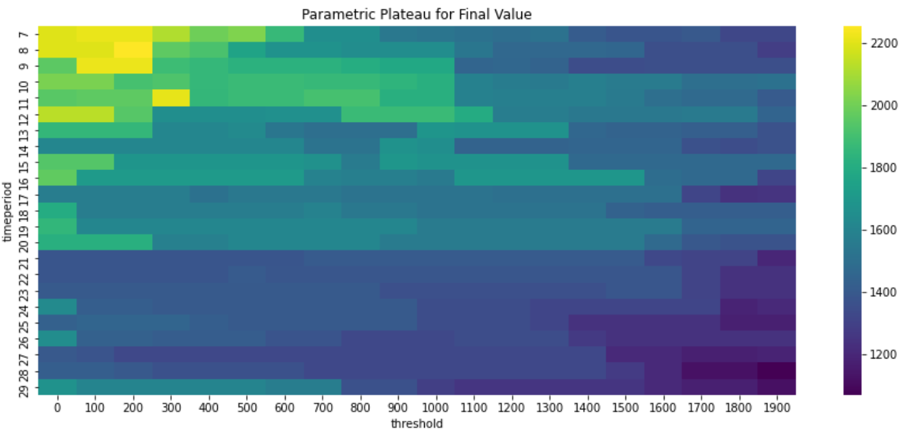
CSCV
I use combinatorially symmetric cross validation (CSCV) in particular to implement Sharpe ratio-based strategy performance testing. The probability of backtest overfit, performance degradation, probability of loss, and stochastic dominance are computed and visualised. The Sharpe ratio was employed as a performance metric by the writers in the reference. Other measurements are appropriate based on the assumptions made in the research.
RSI
WILLR
AROONOSC
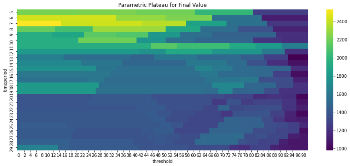
BOP
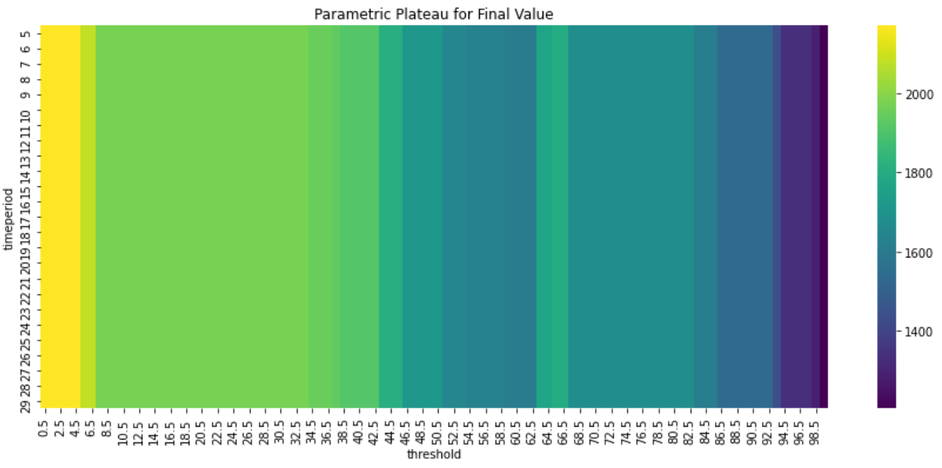
MMI
CCI
MACD
MFI
MOM
ULTOSC
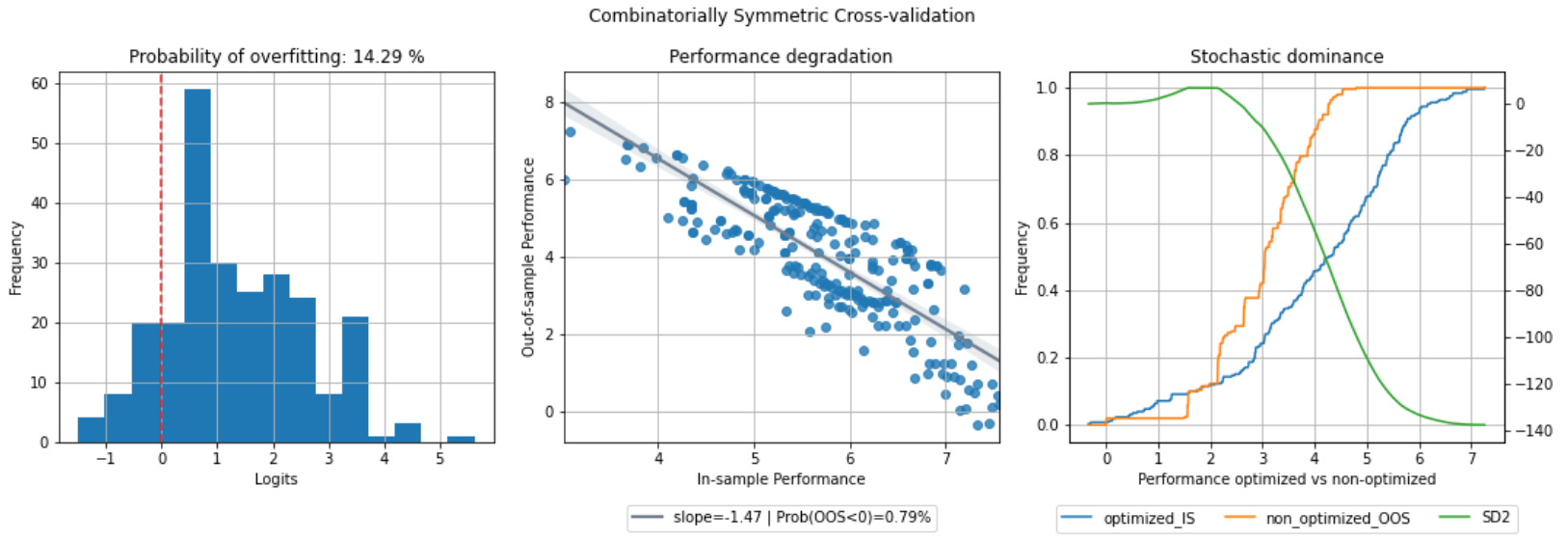
PBO Results
PoL indicates Probability of Loss and PBO indicates Probability of Backtest Overfitting. Slope is for the measurement of Performance Degradation.
| Technical Indicator | PBO [%] | PBO (without LM) [%] | PoL [%] | PoL (without LM) [%] | Slope |
|---|---|---|---|---|---|
| BERT + RSI | 12.70 | 17.86 | 3.66 | 0.00 | -0.52 |
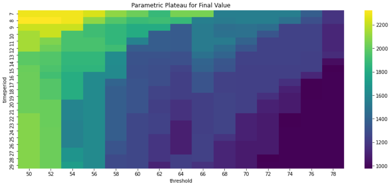
| BERT + WILLR | 6.75 | 26.98 | 1.98 | 17.34 | -1.71 |
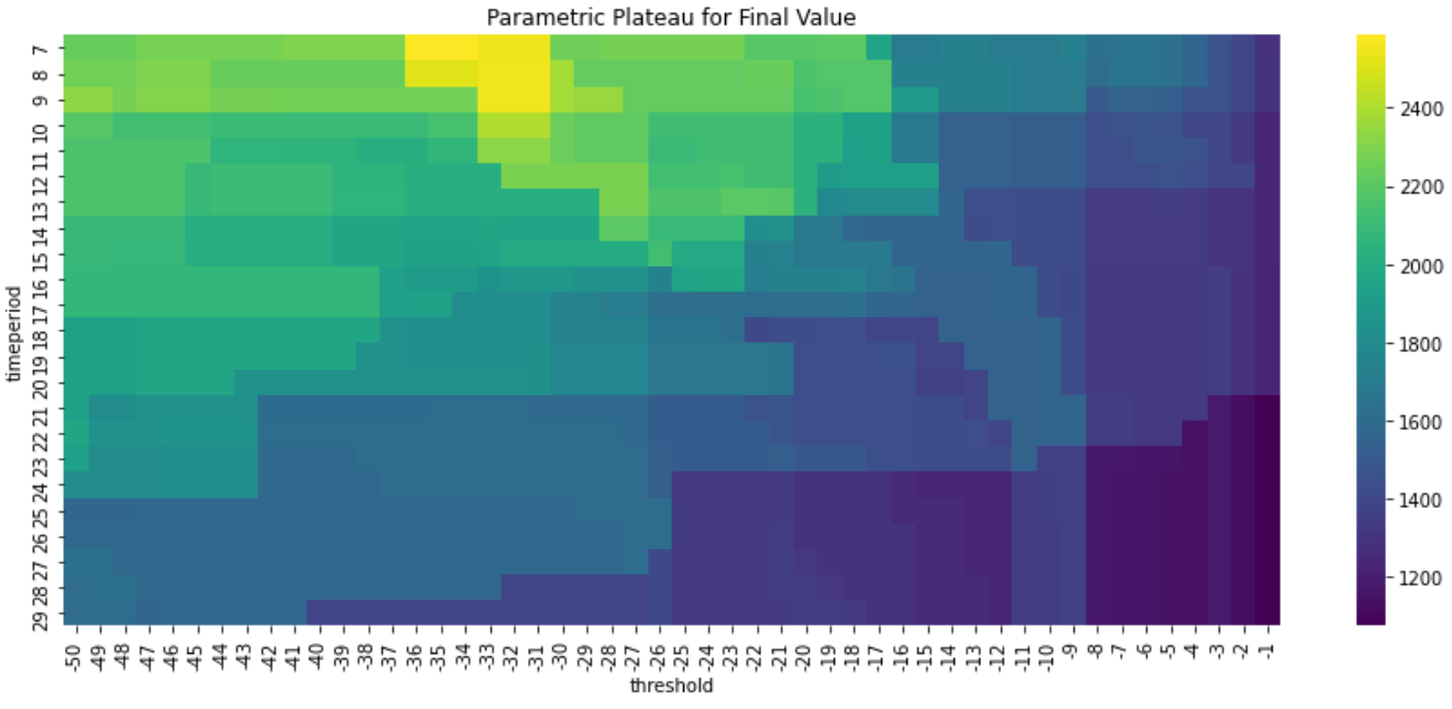
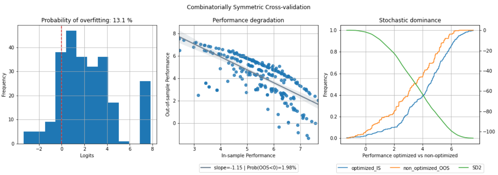
| BERT + AROONOSC | 13.10 | 45.63 | 1.98 | 2.38 | -1.15 |
| BERT + BOP | 54.76 | - | 0.00 | - | -0.83 |
| BERT + MMI | 22.22 | 23.02 | 12.05 | 0.40 | -0.76 |
| BERT + CCI | 3.57 | 48.02 | 3.57 | 8.73 | -1.48 |
| BERT + MACD | 11.51 | - | 8.10 | - | -0.27 |
| BERT + MFI | 7.54 | 46.03 | 5.56 | 6.35 | -1.41 |
| BERT + MOM | 22.62 | 29.76 | 1.59 | 5.95 | -1.38 |
| BERT + ULTOSC | 14.29 | - | 0.79 | - | -1.47 |
Conclusion
When employing numerous criteria to make trading decisions, especially when combining NLP-based indicators with technical indicators, the profit and sharpe ratio can be greatly increased, and drawdown can be significantly decreased.